Constraints on credit, consumer
behaviour and the dynamics of wealth
Gomes, Orlando
Escola Superior de Comunicação Social - Instituto Politécnico de
Lisboa
January 2007
Online at
https://mpra.ub.uni-muenchen.de/2886/
Constraints on Credit, Consumer Behaviour and the
Dynamics of Wealth
Orlando Gomes
∗Escola Superior de Comunicação Social [Instituto Politécnico de Lisboa] and Unidade de Investigação em Desenvolvimento Empresarial [UNIDE/ISCTE].
- January, 2007 -
Abstract: This note develops a simple macro model where the pattern of wealth
accumulation is determined by a credit multiplier and by the way households react to short run fluctuations. In this setup, long term wealth dynamics are eventually characterized by the presence of endogenous cycles.
Keywords: Credit constraints, Financial development, Consumer confidence, Endogenous
business cycles, Nonlinear dynamics.
JEL classification: O41, E32, C61.
∗ Orlando Gomes; address: Escola Superior de Comunicação Social, Campus de Benfica do IPL,
1549-014 Lisbon, Portugal. Phone number: + 351 93 342 09 15; fax: + 351 217 162 540. E-mail:
1. Introduction
The relation between collateral requirements or credit constraints and business
cycles is a relevant theme of discussion in today’s macroeconomic analysis. This
subject has gained visibility with the contributions of Bernanke and Gertler (1989) and
Kyotaki and Moore (1997), and was further developed with the work of Aghion,
Bacchetta and Banerjee (2001, 2004), Demirguç-Kunt and Levine (2001), Amable,
Chatelain and Ralf (2004), Aghion, Angeletos, Banerjee and Manova (2005) and
Caballé, Jarque and Michetti (2006), among others. The basic intuition underlying the
previous references is that markets where firms face some degree of credit constraints
are markets where investment is strongly pro-cyclical and, thus, main economic
aggregates will be subject to amplified volatility that tends to persist over time.
Basically, the lesson one withdraws from this literature is that cycles are more likely to
be observed for specific levels of financial development than for others.1 For instance,
Caballé, Jarque and Michetti (2006), hereafter CJM, conclude that stability is found for
low and high levels of financial development, while for intermediate levels endogenous
business cycles dominate.
In this note, we recover the CJM model to present an alternative approach to the
formation of endogenous cycles for intermediate levels of financial development.
Basically, we consider a same scenario as the previous authors, but with two important
changes: first, we consider physical capital as the unique production input (we ignore
the country specific input with a constant supply assumed in the referred model);
second, we introduce a mechanism through which households respond to short run
wealth deviations from a potential wealth level. Furthermore, the analysis will be
undertaken under an endogenous growth framework, in the sense that it assumes an AK
production function.
This note is organized as follows. Section 2 presents the model’s structure, section
3 discusses local dynamics; section 4 characterizes global dynamics and section 5
concludes.
2. The Structure of the Model
Consider a competitive economy populated by a large number of households and
firms. Firms produce a tradable good under an AK production function, yt=Akt, with
A>0 a technology index and kt, yt the per capita levels of physical capital and output in
moment t.2 We assume that capital fully depreciates after one period and, hence, it=kt,
with it per capita investment. Households have the possibility to lend their financial
resources directly to firms if the marginal productivity of capital (A) is above the
economy’s nominal interest rate (r); hereafter, we impose this constraint on parameters:
A>r.
If the credit market is subject to some kind of imperfection, firms’ financial
resources (that we designate by wealth) will serve as collateral for the loans, and thus
firms cannot borrow an amount over
µ
wt, with wt the level of per capita wealth andµ
acredit multiplier that reflects the degree of financial development of the economy.
Households and firms agree on applying to the productive projects the largest amount of
credit that can be subject to transaction, and thus investment in moment t corresponds to
it=(1+
µ
)⋅
wt. Finally, the structure of the model is complete with a difference equationreflecting wealth dynamics,
t t t
t y r w c
w+1 = −
µ
− , w0 given. (1)
Equation (1) states that wealth in moment t+1 corresponds to income in t, less the
cost of debt and less the resources allocated to consumption (ct is per capita
consumption). In the CJM model, ct corresponds to a constant fraction of income less
debt payment. We generalize this assumption by considering that the marginal
propensity to consume depends on the observable difference between effective levels of
wealth and expected or potential wealth. In practice, agents react to business cycles by
adopting the following rule: the higher the level of last period’s wealth relatively to the
benchmark level of wealth, the more optimistic households will be and, accordingly, the
higher will be the share of consumption out of income. In other words, low (high) levels
of observed accumulated wealth relatively to a benchmark level will imply a
precautionary (confident) behaviour that is translated on a higher (lower) savings rate.
Formally, we consider ct =c⋅(yt −r
µ
wt)⋅g(wt−1), c∈(0,1) and g(wt) a positive,continuous and differentiable function, with g’>0. Consider *
t
w as the potential level of
wealth; this is supposed to represent a wealth trend that grows at a same rate,
γ
, for all t.
Thus, function g will be such that ( )| = *=1 t t w w t w
g , ( )| > *>1
t t w
w t
w
g and ( )| < *<1
t t w w t w g .
The following functional form fulfils the required properties:
a t t t w w w g = * )
( , a>0.
The reduced form of the dynamic system is straightforward to obtain given the
previous information,
[
]
ta t t t w w w c r A A w ⋅ ⋅ − ⋅ ⋅ − + = − − + * 1 1
1 ( )
µ
1 (2)Because production is subject to constant marginal returns, all relevant variables
(kt, yt, it, ct and wt) grow at a constant positive rate in the steady state. Let this rate be
γ
,and thus we define variable t t
t w w ) 1 ( ˆ
γ
+≡ and constant wt t
w ) 1 ( ˆ * *
γ
+≡ . Effective wealth
grows at a same rate as potential wealth in the steady state, but before this long run
result is eventually accomplished, the growth rates might differ. Rewriting (2),
t a t t w w w c r A A w ˆ ˆ ˆ 1 1 ) (
ˆ *1
1 ⋅
⋅ − ⋅ + ⋅ − + = −
+
γ
µ
(3)Equation (3) has a unique equilibrium point: *
/ 1 ˆ ) ( 1 1 1 w r A A c w a ⋅ ⋅ − + + − ⋅ =
µ
γ
.This result allows us to state the following proposition,
Proposition 1: The wealth model, with credit constraints and consumption
reaction to deviations from last period’s potential wealth, reveals that the higher is the
level of financial development of the economy, the larger will also be the amount of
accumulated wealth, in the steady state.
Proof: Take the steady state expression for the wealth variable and compute
derivative
µ
µ = ∂∂
w
[
]
⋅ − + − ⋅ + ⋅ ⋅ ⋅ − + + − ⋅ ⋅ = − 2 1 * ) ( ) ( ) 1 ( 1 ) ( 1 1 1 ˆµ
γ
µ
γ
µ r A A r A c r A A c a w w a a. Because this is a
positive value, one infers that the accumulated level of wealth is positively correlated
with financial development (measured by the credit multiplier parameter,
µ
)Note, relatively to the steady state value, that to guarantee w >0, the following
inequality must hold: A+(A−r)⋅µ >1+γ . This condition imposes a floor to the value
of the credit parameter:
r A A − − + > γ
µ 1 is the minimal requirement for the economy to be
able to accumulate wealth.
3. Local Dynamics
In this section, we address the dynamics of equation (3) in the neighbourhood of
point w. This requires defining variables w~t ≡wˆt −w and ~zt ≡wˆt−1 −w. With these
variables, we turn equation (3) into a two equation system with two endogenous
variables and just one time lag,
= − + ⋅ + ⋅ − ⋅ + ⋅ − + = + + t t t a t t w z w w w w w z c r A A w ~ ~ ) ~ ( ˆ ~ 1 1 ) ( ~ 1 * 1 γ µ (4)
Around the balanced growth path, system (4) takes the linearized form
⋅ + + − ⋅ − + ⋅ − = + + t t t t z w r A A a z w ~ ~ 0 1 1 ) 1 ( ) ( 1 ~ ~ 1 1
γµ γ (5)
Note that the steady state values of variables w~ and t z~ are, in both cases, 0. Proposition t
Proposition 2: The wealth model under analysis is locally stable for − − + ⋅ + − − + ∈ r A A a a r A
A (1 )
1
;
1
γ
γ
µ
; whenr A A a a − − + ⋅ + = ) 1 ( 1
γ
µ
, the systemundergoes a Neimark-Sacker bifurcation.
Proof: The Jacobian matrix in (5) has a positive determinant,
γ
µ
γ
+ + − ⋅ − + ⋅ = 1 ) 1 ( ) ( )
(J a A A r
Det , and its trace is Tr(J)=1. Thus, stability conditions
1-Tr(J)+Det(J)>0 and 1+Tr(J)+Det(J)>0 are always satisfied. The only possible
bifurcation occurs when the eigenvalues of the matrix are a pair of complex conjugate
values with modulus equal to one, which is equivalent to say that Det(J)=1. The
equality expression in the proposition is determined by solving this last condition in
order to
µ
. Stability requires 1-Det(J)>0From proposition 1, we have concluded that the less constrained credit is, the
larger is the amount of wealth the economy accumulates in the long run, while from
proposition 2 one observes that there is a stability ceiling: if freedom to offer credit is
too high, the guarantee that the steady state level of wealth is achieved vanishes.
Therefore, one can interpret this theoretical structure as indicating both the advantages
of financial development and of financial responsibility, in the sense that excessive
credit may disrupt the financial system as agents fail to pay back the large amount of
resources they have borrowed.
Local dynamics conceal meaningful features of the model. First, cycles appear to
be absent. The theory on nonlinear dynamics points to the eventual presence of cycles
after a bifurcation. In our concrete system, we should expect to effectively encounter a
fixed point in the stability area identified in proposition 2, and a-periodic motion after
the bifurcation and before instability truly sets in. This becomes evident with the global
analysis of the following section. Second, the global analysis of this specific model will
show that some points of stability are present in the locally unstable area, a result that
can be used to justify a same kind of conclusion as the one in the CJM model: financial
instability (cycles) occurs for intermediate levels of development, while stability is
4. Global Dynamics
To address global dynamics consider an array of reasonable parameter values:3 [A;
c;
γ
; r; w*; a]=[1; 0.75; 0.04; 0.03; 1; 0.7] and let us electµ
as the bifurcationparameter. In this particular case, the system is stable for 0.041<
µ
<1.573.Figure 1 shows the bifurcation diagram; a bifurcation, that occurs for
µ
=1.573,separates an area of stability from an area where invariant cycles can be observed. After
the region where endogenous cycles are evidenced, it follows a state where stability and
instability alternate. Recall that w~ is a variable that was modified twice: first, it was t
detrended and, then, adjusted to obtain a balanced growth path where the variable takes
the value zero. In the long run, the original variable wt grows exponentially, with a
detrended value equal to w.
*** Figure 1 here ***
To understand that this framework produces everlasting endogenous business
cycles for specific values of the credit parameter, we present a time series of w~ in t
figure 2. The Neimark-Sacker bifurcation, or Hopf bifurcation in discrete time, is able to
generate a kind of dynamics that reproduces considerably well real world business
cycles, in the sense that several consecutive periods of increasing wealth are followed
by some periods where there is a slowdown on the growth of wealth, and so on.
*** Figure 2 here ***
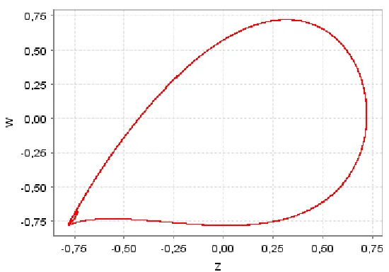
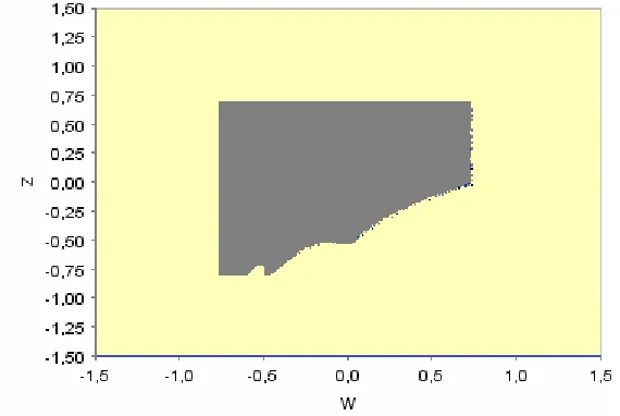
To close the graphical presentation, and taking the same value of
µ
as in figure 2,we draw an attractor that reveals the long run relation between w~t−1 and w~ (figure 3) t
and the basin of attraction that furnishes the set of initial points that allow for a
convergence towards the long run attractor (figure 4).
*** Figures 3 and 4 here ***
5. Conclusions
3 In particular, observe that the marginal propensity to consume corresponds to 75% of income, that the
Following the literature on credit constraints and business cycles, we have
considered a basic AK endogenous growth model, where financial development is
addressed through a credit multiplier and where economic agents take consumption
decisions by weighting last period’s difference between observed and potential wealth
(if this difference is positive, consumers optimism rises and they will increase their
consumption share of income; with a negative difference, households become less
enthusiastic about consumption and they will prefer to increase the marginal propensity
to save, as a precautionary measure).
The proposed setup is able to elucidate about two important points:
i) As the financial development level rises, per capita wealth, in the steady state,
also increases;
ii) Fixed point stability is found for low levels of financial development (and, thus,
low levels of accumulated wealth); an intermediate level of the credit multiplier allows
to identify a-periodic cycles generated through a Neimark-Sacker bifurcation; and high
levels of financial development are characterized by a scenario where stability and
instability alternate.
The instability result for high levels of the credit multiplier adds a new feature
relatively to the CJM model: too high credit multipliers, associated to loans with no
collateral, imply a high risk in the credit market, in the sense that borrowers may not
carry out their debt payment obligations. In this case, instability may be interpreted as a
scenario of financial crisis that imposes the need to restore a certain ceiling on the level
of available credit.
References
Aghion, P.; G. M. Angeletos; A. Banerjee and K. Manova (2005). “Volatility and
Growth: Credit Constraints and Productivity-Enhancing Investment.” NBER
working paper nº 11349.
Aghion, P.; P. Bacchetta and A. Banerjee (2001). “Currency Crises and Monetary
Policy in an Economy with Credit Constraints.” European Economic Review, vol.
45, pp. 1121-1150.
Aghion, P.; P. Bacchetta and A. Banerjee (2004). “Financial Development and the
Instability of Open Economies.” Journal of Monetary Economics, vol. 51, pp.
Amable, B.; J. B. Chatelain and K. Ralf (2004). “Credit Rationing, Profit Accumulation
and Economic Growth.” Economics Letters, vol. 85, pp. 301-307.
Bernanke, B. and M. Gertler (1989). “Agency Costs, Net Worth, and Business
Fluctuations.” American Economic Review, vol. 79, pp. 14-31.
Caballé, J.; X. Jarque and E. Michetti (2006). “Chaotic Dynamics in Credit Constrained
Emerging Economies.” Journal of Economic Dynamics and Control, vol. 30, pp.
1261-1275.
Demirguç-Kunt, A. and R. Levine (2001). Financial Structure and Economic Growth.
Cambridge, MA: MIT Press.
Kyotaki, N. and J. Moore (1997). “Credit Cycles.” Journal of Political Economy, vol.
Figure 1 – Bifurcation diagram (1.5<µµµµ<2).
Figure 2 – Time series (µµµµ=1.891).