SOLVING ECONOMIC DISPATCH PROBLEM USING PARTICLE SWARM OPTIMIZATION BY AN EVOLUTIONARY TECHNIQUE FOR INITIALIZING PARTICLES

794

TRACKING CONTROL FOR WHEELED MOBILE ROBOTS

USING NEURAL NETWORK MODEL ALGORITHM

CONTROL

YUANLIANG ZHANG

1

School of Mechanical Engineering, Huaihai Institute of Technology, Lianyungang 222005, Jiangsu, China

ABSTRACT

This paper proposed a neural network model algorithm control (NNMAC) method for the path tracking control of differentially steered wheeled mobile robots (WMRs) subject to nonholonomic constraints. The model algorithm control (MAC) is a one-step-ahead predictive controller, in which the control law is obtained by minimizing the output error. The MAC method needs the well known model of the controlled system to design the controller. But sometimes it is difficult to get the accurate model of the controlled system or the model of the controlled system is not good because of the inside and outside disturbances and unknown parameters. Neural network has the ability to estimate the nonlinear system’s model and its corresponding inverse model. In this paper the NNMAC method which combines two neural networks and MAC method is proposed to do the path tracking control of a wheeled mobile robot. Some simulations are conducted to show the performance and feasibility of the proposed control strategy. In these simulations the WMR is controlled to track two difference reference paths such as the circular shape path and the “8” shape path.

Keywords: Neural Network, Model Algorithm Control, Mobile Robot

1. INTRODUCTION

The differentially steered wheeled mobile robot which possesses the advantages of high mobility, high traction with pneumatic tires, and a simple wheel configuration is a kind of nonholonomic system [1]. Nonholonomic systems most commonly arise in finite dimensional mechanical systems where constraints are imposed on the motions that are not integrable. In the case of the differentially driven WMRs, the constraints involved are based on the assumption that there is no slipping of the wheels. There are two fundamental statuses in controlling a mobile robot: posture stabilization and path tracking. The aim of posture stabilization is to stabilize the robot to a reference point, while that of path tracking is to have the robot follow a reference path. For WMRs, path tracking is easier to achieve than posture stabilization. This comes from the assumption that the wheels make perfect contact with the ground, resulting in nonholonomic constraints.

The tracking control of nonholonomic mobile robots aims at getting them to track a given time varying path (reference path). It is a fundamental motion control problem and has been intensively investigated in the robotic domain [2-5]. Felipe et al. [6] proposed an adaptive controller for

autonomous mobile robot trajectory tracking. Ye [7] proposed a tracking control approach for nonholonomic mobile robots by integrating the neural network into the backstepping technique. Sun [8] designed a trajectory tracking controller for the mobile robot based on pole assignment approach. Park et al. [9] solved the point stabilization of mobile robots via state-space exact feedback linearization.

ISSN: 1992-8645 www.jatit.org E-ISSN: 1817-3195

795 weight adaptation. We propose in this paper a MAC method using back propagation (BP) neural networks to do the path tracking control of a WMR. Simulations are conducted to show the performance and feasibility of the proposed control method.

2. MAC CONTROL METHOD

Consider the nonlinear systems described by a discrete-time state-space model of the form:

( 1) [ ( ), ( )]

( ) [ ( )]

m m

m m

x k x k u k r

y k h x k

+ = Φ −

= (1)

where x denotes the state variables,udenotes the input,y represents the output to be controlled and the subscript m is added to indicate the estimates of

x

and

y

obtained in the model simulations and differentiate the measured x and y .Φ( , )x u is an analytic vector function on X U× , andh x is an ( ) analytic scalar function onX. Here,ris the relative order of the system (1), i.e.ris the smallest number of sampling periods after which the manipulated inputuaffects the outputy.

The online simulation of the model described by Eq. (1) can be used to predict the future changes in the outputyas follows:

1

2

1

1

( 1) ( ) [ ( )] [ ( )]

( 2) ( ) [ ( )] [ ( )]

...

( 1) ( ) [ ( )] [ ( )]

( ) ( ) [ [ ( ), ( )]}

[ ( )]

m m m m

m m m m

r

m m m m

r

m m m

m

y k y k h x k h x k

y k y k h x k h x k

y k r y k h x k h x k

y k r y k h x k u k

h x k

−

−

+ − = −

+ − = −

+ − − = −

+ − = Φ

−

(2)

Here the following notation is used:

[

]

0

1

( ) ( )

( ) ( , ) , 1,..., 1

l l

h x h x

h x h− x u l r

 ₌

 

= Φ = −

 (3)

System (1) has the relative orderrmeans that

(

)

(

)

1

( , )

0, 0,1,..., 2;

( , ) 0

l

r

h x u

l r

u

h x u

u − ∂ Φ = = − ∂ ∂ Φ ≠ ∂ (4)

Furthermore, the following relations will hold:

1 ( ) [ ( )], ( ) { [ ( ), ( )]} 0,..., 1 l r

y k l h x k

y k r h x k u k

l r

−

 _{+ =}

 

+ = Φ



= −

(5)

Therefore,r is the smallest number of sampling periods after which the manipulated input u affects the output y . With a finite relative

order r ,

(

)

1 _{( , )}

0 r

h x u

u

−

∂ Φ

≠

∂ implies that the

algebraic equation:

1

[ ( , )] r

h − Φ x u = y (6) is locally solvable in u . The corresponding implicit function is denoted by:

0

( ) ( ( ), ( ))

u k = Ψ x k y k+r (7)

and is assumed to be well-defined and unique onX×h X( ).

When the predicted changes shown in Eq. (2) are added to the measured output signaly , one obtains the following “closed-loop” predictions of the output:

1

2

1

1

ˆ( 1) ( ) [ ( )] [ ( )]

ˆ( 2) ( ) [ ( )] [ ( )]

...

ˆ( 1) ( ) [ ( )] [ ( )]

ˆ( ) ( ) [ [ ( ), ( )]]

[ ( )] m m m m r m m r m m

y k y k h x k h x k

y k y k h x k h x k

y k r y k h x k h x k

y k r y k h x k u k

h x k

−

−

+ = + −

+ = + −

+ − = + −

+ = + Φ

−

(8)

where y kˆ( ) represents a prediction of the outputy k . ( )

Here a desirable value, y , of the output at _d the(k+r)thtime step is designed by:

ˆ

( ) (1 ) ( ) ( 1)

d sp

y k+ = −r α y k +αy k+ −r (9)

whereα is a tunable filter parameter such that

0< <α 1 andy is the set-point value. Equation (9) is _sp

referred to as the “reference trajectory” in the MAC literature.

One can derive a nonlinear MAC controller by requesting that the output prediction match the reference path in the sense of minimizing the performance index of Eq. (10):

2

( )

ˆ

min[ _d( ) ( )]

796

1

( )

1 2

min{(1 ) ( ) { [ ( ), ( )]} [ ( )] (1 ) [ ( )]}

r m u k

r

m m

e k h x k u k

h x k h x k

α

α α

−

−

− − Φ

+ + − (11)

wheree(k)=y_sp( )k −y k( ).

In the absence of input constraints, this minimization problem is trivially solvable. Inputu k is the solution of the nonlinear algebraic ( ) equation:

(

) (

)

1

( ( ), ( )) ( ), ( )

r

m m

h− Φ x k u k =b x k e k (12) whereb x e( , )=αhr−1( )x + −(1 α)

(

h x( )+e

)

.

Recalling the definition of

Ψ

₀ (Eq. (7)), the solution can be represented as:

(

)

(

)

0

( ) _m( ), _m( ), ( )

u k = Ψ x k b x k e k (13)

Therefore, the derived control law is given by Eq. (13).

3. MAC USING NEURAL NETWORKS

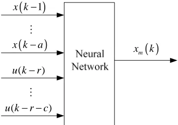
Two neural networks, NN1 and NN2, are employed in deriving the NNMAC method. In this proposed control scheme, the neural network NN1 is trained as the model of the controlled system and the neural network NN2 is trained to produce the control inputs. In this paper, we adopt the BP neural network and use the NNARX (AutoRegressive External input) model structure as the structure of the two neural networks. For this model structure, the inputs of the neural network are the past data of the system output and input of the system. Figure 1 shows the configuration of the BP neural network. Figure 2 depicts the NNARX model structure. The parameters

a

and

c

are the numbers of past data of the system output and control input, respectively.

x

is the estimated system’s output,

u

is the system’s input,

x

_m is the neural network’s output and

r

is the relative order of the nonlinear system.

1

ϕ

p

ϕ

pl

M Mlj

1 m

x

mj

[image:3.612.327.508.287.414.2]

x

Figure 1: Configuration Of The BP Neural Networks

(

1

)

x k

−

(

)

x k

−

a

(

)

u k

−

r

(

)

u k

− −

r

c

M

M

( )

m

x

k

Figure 2: The NNARX Model Structure

ISSN: 1992-8645 www.jatit.org E-ISSN: 1817-3195

797 system output and input. The error signal used to adjust the weights of the neural network NN2 is the difference between the controlled system’s input and the neural network’s output. Figure 4 shows the structure used to train the neural network NN2.

( ) u k−r

Controlled System

NN1 Neural Network

( ) x k

+ −

E

( )

m

x k

2

q−

3

q−

3

q−

2

q−

1

q−

1

[image:4.612.91.296.160.502.2]

q−

Figure 3: Structure Used To Train The Neural Network Nn1

+ −

1

q−

2

q−

3

q−

3

q−

2

q−

4

q−

5

q−

E ( )

u k x k( +r)

'( ) u k

Figure 4: Structure Used To Train The Neural Network Nn2

For MAC method the control input can be calculated using Eq. (13). In Eq. (13) the function

0

Ψ is obtained from Eq. (7) andx_m( )k comes from Eq. (1). Analogizing to the MAC method presented in Section 2, the NNMAC method presented in Section 3 uses the two neural networks, NN1 and NN2, to do the control job. In this case it is assumed that the model and inverse model of the controlled system are hard to obtain. This means that Eq. (1) and Eq. (7) are unknown. In this case the neural network NN1 is trained to estimate the controlled system’s model Eq. (1) to

generatex_m( )k ; and the neural network NN2 is trained to estimate the function ofΨ₀ . Then the control input can be generated by using the neural networks NN1 and NN2. The diagram of the proposed control system is shown in Figure 5.

u y

m x sp

y

( ) ( ),

[image:4.612.321.514.168.235.2]

m b x_ k e k_

Figure 5: Principle Of The Nnmac Control System

4. SIMULATION

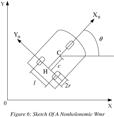
The proposed NNMAC control method can be used to do the path tracking control of the WMR. Consider a nonholonomic WMR with two differentially steered wheels, as shown in Figure 6. This WMR has two driving wheels (radius

r

) and one caster. PointH x( _H,y_H)defines the intersection of the axis of symmetry with the driving wheel axis, and is assumed to be the origin of the coordinate frame{X_H,Y_H}. Point C x y( ,_{c c}) is the center of mass of the mobile robot. Length

c

is the distance between pointH and point C , and l is the length of the rear wheel axis.

H

X

H

Y

H C

θ

l _2r

[image:4.612.324.510.452.643.2]

c

Figure 6: Sketch Of A Nonholonomic Wmr

798 the proposed control law to demonstrate its effectiveness. First a circular reference path is used to do the simulation. The tracking performance of the NNMAC controller for the circular reference path is shown in Figure 7. And Figure 8 shows the linear and angular velocities of the mobile robot in this case.

-1.5 -1 -0.5 0 0.5 1 1.5 -1.5

-1 -0.5 0 0.5 1 1.5

x (m)

y

(

m

)

[image:5.612.322.514.85.272.2]

reference path tracking path

Figure 7: Tracking Performance In The Case Of Circular Reference path

0 10 20 30 40 50 60

0 1 2 3 4

t (s)

v

(

m

/s

)

0 10 20 30 40 50 60

-1 0 1 2 3 4

t (s)

w

(

ra

d

/s

[image:5.612.103.283.190.352.2]

)

Figure 8: Linear And Angular Velocities In The Case Of Circular Reference Path

-0.8 -0.6 -0.4 -0.2 0 0.2 0.4 0.6 0.8 -1

-0.8 -0.6 -0.4 -0.2 0 0.2 0.4 0.6 0.8 1

x (m)

y

(

m

)

[image:5.612.323.505.394.555.2]

reference path tracking path

Figure 9: Tracking Performance In The Case Of “8” Shape Reference Path

Next we choose the reference path as an “8” shape path. The tracking performance of the NNMAC controller for the “8” shape reference path is shown in Figure 9. And Figure 10 shows the linear and angular velocities of the mobile robot in this case.

0 10 20 30 40 50 60 70 80 0

0.5 1 1.5

v

(

m

/s

)

t (s)

0 10 20 30 40 50 60 70 80 -1

-0.5 0 0.5 1 1.5

t (s)

w

(

m

/s

)

Figure 10: Linear And Angular Velocities In The Case Of “8” Shape Reference Path

From the accurate performance of the simulation it can be seen that the proposed NNMAC control method can provide a good control result for the path tracking of the WMRs.

5. CONCLUSION

[image:5.612.103.283.402.565.2]

ISSN: 1992-8645 www.jatit.org E-ISSN: 1817-3195

799 wheeled mobile robot. MAC is a one-step-ahead predictive controller, in which the control law is obtained by minimizing the output error. Two neural networks, NN1 and NN2, are introduced to cooperate with the MAC control method. The neural network NN1 was trained as the model of the controlled system and the neural network NN2 was trained to generate the control inputs. The numerical simulation is conducted to show the promise of the proposed NNMAC control method in terms of tracking performance. In the simulation a circular reference path and an “8” shape reference path are used.

ACKNOWLEDGEMENTS

This paper is supported by Huaihai Institute of Technology Bringing in Talent Research Starting Fund project (KQ10125).

REFERENCES:

[1] Yulin Zhang, Daehie Hong, Jae H. Chung, Steven A. Velinsky, “Dynamic model based robust tracking control of a differentially steered mobile robot”, Proceedings of the 1998

American Control Conference, IEEE

Conference Publishing Services, June 21-26, 1998, pp. 850-855.

[2] Omid Mohareri, Rached Dhaouadi, Ahmad B. Rad, “Indirect adaptive tracking control of a nonholonomic mobile robot via neural networks”, Neurocomputing, Vol. 88, No. 5, 2012, pp. 54-66.

[3] George P. Moustris, Spyros G. Tzafestas, “Switching fuzzy tracking control for mobile robots under curvature constraints”, Control Engineering Practice, Vol. 19, No. 1, 2011, pp. 45-53.

[4] K.D. Do, “Output-feedback formation tracking control of unicycle-type mobile robots with limited sensing ranges”, Robotics and Autonomous Systems, Vol. 57, No. 1, 2009, pp. 34-47.

[5] Markus Mauder, “Robust tracking control of nonholonomic dynamic systems with application to the bi-steerable mobile robot”, Automatica, Vol. 44, No. 10, 2008, pp. 2588-2592.

[6] Felipe N. Martins, Wanderley C. Celeste, Ricardo Carelli, Mário Sarcinelli-Filho, Teodiano F. Bastos-Filho, “An adaptive dynamic controller for autonomous mobile robot trajectory tracking”, Control Engineering Practice, Vol. 16, No. 11, 2008, pp. 1354-1363. [7] Jun Ye, “Tracking control for nonholonomic

mobile robots: integrating the analog neural network into the backstepping technique”, Neurocomputing, Vol. 71, No. 16-18, 2008, pp. 3373-3378.

[8] Shuli Sun, “Designing approach on trajectory-tracking control of mobile robot”, Robotics and Computer-Integrated Manufacturing, Vol. 21, No. 1, 2005, pp. 81-85.

[9] Kyucheol Park, Hakyoung Chung, Jang Gyu Lee, “Point stabilization of mobile robots via state-space exact feedback linearization”, Robotics and Computer-Integrated Manufacturing, Vol. 16, No. 5, 2000, pp. 353-363.

[10] Qijun Xia, Ming Rao, Jixin Qian, “Model algorithm control for paper machines”, Proceedings of Second IEEE Conference on

Control Applications, IEEE Conference