New Task Domain Propagators with Polynomial Complexity for Resource Constrained Project Scheduling Problem

2018 IX International Conference on Optimization and Applications (OPTIMA 2018) ISBN: 978-1-60595-587-2

New Task Domain Propagators with Polynomial Complexity for

Resource-Constrained Project Scheduling Problem

Dmitry ARKHIPOV

, Olga BATTAÏA

_{, Alexander LAZAREV}

_,

German TARASOV

_{, and Ilia TARASOV}

Department of Complex Systems Engineering, ISAE-SUPAERO, Université de Toulouse, 10 avenue Edouard Belin - BP 54032 - 31055 Toulouse Cedex 4, France

V.A. Trapeznikov Institute of Control Sciences of Russian Academy of Sciences, Moscow, Russia Lomonosov State University, Moscow, Russia

National Research University Higher School of Economics, Moscow, Russia Moscow Physical and Technical Institute (State University), Dolgoprudnyi, Russia

Corresponding author

Project scheduling, Constraint programming, Scheduling, RCPSP, Task domain propagator

We consider a classic Resource-Constrained Project Scheduling Problem (RCPSP) which is known to be NP-hard. For defined project deadline T , each task of the pro ject can be associated with its temporal domain – a time interval in which this task can be processed. In this research, we adopt existing resource-based methods of task domain propagation to generalized statement with time-dependent resource capacity and show how to improve its propagation effi- ciency. We also present new polynomial-time algorithms (propagators) to tighten such temporal task domains in order to make the optimization problem easier to solve. Moreover, we show how these propagators can be used to calculate lower bound on project makespan.

Introduction

The Resource Constrained Project Scheduling Problem (RCPSP) is a well-known scheduling theory problem. This problem is strongly NP-hard [8]. This paper is focused on constraint pro- gramming resource-based methods to solve RCPSP.

Constraint programming approaches are widely used to solve scheduling problems including RCPSP. This approach is used in well-known solvers, i.e. IBM ILOG CP Optimizer, Choco, MiniZinc, Gecode, etc. Propagators can also be used as a powerful data pre-processing tool, to make task domains tighter and add new precedence relations.

This paper is organized as follows. In the section 2 the existing resource-based propagators for RCPSP are reviewed. Problem statement and data preprocessing procedures are presented in sections 3 and 4 respectively. In the section 5 we show how to adapt existing propagators to generalized RCPSP statement with time-dependent resource capacity. In sections 6 and 7 approaches to bound resource capacity function and pro ject makespan are presented. By the section 8 we conclude.

1

2

3

4

5

Keywords:

Abstract.

State of the Art

There is a wide range of Constrained Programming techniques which can be applied to find an optimal/suboptimal solution of RCPSP or to make the problem easier to solve.

Some methods allow to add new precedence relations between tasks. In [18] and [5] the term of disjunctive graph was introduced and used to solve scheduling problems.

This research is focused on resource-based constraints. Let us briefly list them, the discussion of the most important for us will be given in section 5. A lot of constraints can be obtained by considering Cumulative Scheduling Problem (CuSP) – a single-resource version of RCPSP. Calculation of compulsory parts [12], time-tables [13], resource profile [7], resource histogram [6] allow to clarify resource usage by tasks under any feasible schedule. Time tabling sweep algorithms ([2], [3], [14]) can be used to adjust release times and tails of tasks. In [4] the application of rectangle placement problem to improve Time Tabling technique is presented. Filtering Time Table sweep algorithm with the best theoretical complexity was suggested in [9].

Edge-Finding algorithms ([16], [20], [11]) can be used to make task domains tighter and to avoid resource overloads on time intervals. This approach can be improved by using Extended-Edge-Finding algorithms presented by [15].

One of the advantages of constraint programming method is the possibility to combine different algorithms for more efficient propagation. The synergy of Edge-Finding, Extended Edge Finding and Time Tabling gave very good results obtained in [17].

For other results of using constraint programming to solve scheduling problems, we refer to [1].

Problem Statement

We consider a generalized statement of RCPSP. There is a project which should be finalized in the time horizon T. There is a set of project tasks N, and sets of resources R. In the classic statement the capacity of resource r ∈ R equals to constant value cr. In this paper we consider

task domain propagation methods developed for the classic statement and expand them to the generalized statement of RCPSP, where the capacity of any resource r ∈ R is defined by some non-negative capacity functioncr(t). For any task j ∈N the following attributes are given:

ˆ pj – processing time;

ˆ rj – release time, the earliest possible time when the task j can start the processing;

ˆ hj – tail, which should separate task completion time and project completion time;

ˆ ajr – required amount of resourcer ∈R.

As usual the first and the last tasks of the project are dummy with zero processing times and without any resource requirements, i.e. p0 = pn+1 = 0, r0 = rn+1 = 0, h0 = hn+1 = 0, a0k =

an+1k = 0 for any k ∈ R. Precedence relations with time lags are given by weighted directed

acyclic graph G= (N, E) where E – is the set of edges, defined bu triplets {i, j, eij}, where eij is

the time lag between processing of tasks i∈N and j ∈N.

Schedule π defines start times Sj(π) for each task j ∈ N. Completion time of any taskj ∈N

under scheduleπcan be calculated by the formulaCj(π) =Sj(π) +pj. Scheduleπis called feasible

if the following constraints are satisfied.

1. Release times and tails should be satisfied, i.e. for any j ∈N

[Sj(π), Cj(π))⊆[rj, T −hj).

2. For any resource k ∈R capacity function is not violated for any t, i.e.

X

j∈N|t∈[Sj(π),Cj(π))

ajk ≤ck(t).

3. Precedence relations with time lags should be satisfied. Therefore, any valueeij ∈E implies

that for start times of tasksiandj the inequalitySi(π) +eij ≤Sj(π) holds. Note that values

eij and eji can both belong to E.

The set of all feasible schedules is defined by Π(N, R).

For any j ∈ N we denote the earliest starting time, the earliest completion time, the latest starting time and the latest completion time by estj, ectj, lstj and lctj respectively. By the

problem formulation we know that the taskj should be processed in the time interval [rj, T −hj),

therefore [estj, lctj) ⊆ [rj, T −hj). Introduced notations are more useful, since values rj and hj

are given and estj,ectj, lstj, lctj can be dynamically changed during task domain propagation.

Data Preprocessing

In this part, we make a list of procedures which can improve the efficiency of most of the propagators. From the complexity point of view, it is more efficient to prepare data by applying procedures 1-5 before using propagators. Procedures 4 and 5 can also be used as other propagators: it is reasonable to execute these procedures if something changed to get more adjusted results.

1. For any resource r ∈ R we can create set of tasks Nr ⊆ N which require this resource, i.e.

Nr ={j ∈N|ajr>0}.

2. Longest paths calculation. This takes O(n|E|+n2_{logn) operations, where |E|– number of}

edges in graph G, using algorithm presented in [10].

3. Find the earliest/latest starting/completion times using the formulaeestj =rj,ectj =rj+pj,

lstj =T −hj −pj, lctj =T −hj.

4. If lstj < ectj for any task j ∈N, interval [lstj, ectj) sets a compulsory part of j. This term

was firstly proposed by [12]. The complexity of this procedure isO(1) for one task andO(n) for all tasks of the set N. If all compulsory parts of tasks are calculated we can create a set of tasks NCP ⊆N which compulsory parts are not empty, i.e. NCP ={j ∈N|lstj < ectj}.

During the process of using domain propagators, estj and lctj can be changed and the set

NCP _{can be supplemented.}

5. Calculate highest possible amount of resourcer ∈ R which can be used by non-compulsory parts of taskscn

r(t). This function can be calculated by the formula

cn_r(t) =cr(t)−

X

j∈N:lstj≤t≤ectj

ajr.

For this procedure algorithm presented by [7] can be applied adjusted for piecewise constant resource capacity function. The complexity of this procedure is O(nr +m) operations for

single resource where nr – number of tasks which require resource r during the processing

and m – number of breakpoints of cr(t). If for any task from the set Nr compulsory part

[lstj, ectj) is updated, it is reasonable to recalculate functioncnr(t) to obtain more tight bound

Adapting Existing Propagators to Piecewise-Constant Capacity Function

There are a lot of methods of task domain propagation which are based on resource overload. In this section, we present an adaptation of existing algorithms for the RCPSP generalization with piecewise-constant capacity function and show that in some cases it can improve the efficiency of existing techniques. Presented methods are focused on bounding the earliest starting time, but can be symmetrically used to propagate the latest completion time.

Edge-Finding

The idea of the Edge-Finding algorithm was firstly proposed in [16]. This method can be divided into two parts. In the first part, specific precedence relations Ω_lj for any Ω ⊂ N and j /∈Ω are introduced. Ω_lj means that under any feasible schedule π ∈Π(N, R) the completion time of j is not smaller than the completion time of all tasks of Ω, i.e.

Cj(π)≥max i∈Ω Ci(π).

Fast algorithm to detect all such precedences was presented by Vilim [20]. In the second part for each pair (Ω, j) the following idea is used to tighten the domain of j. Let us consider [estΘ, lctΘ)

– the domain of any Θ ⊆Ω, where estΘ = mini∈Θesti and lctΘ = mini∈Θlcti. Ωlj leads to the

fact that all tasks of Θ have to be completed before Cj(π) which implies that amount of resource

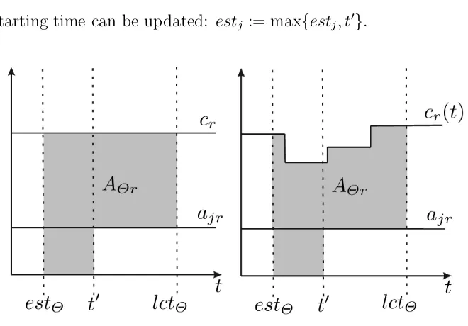
ajr can not be consumed by the tasks of Θ in the interval [Sj(π), lctΘ). LetAΘr =

P

i∈Θair – total

amount of resource r required to process Θ. Therefore (Fig. 1 a)

Sj(π)≥t0 = max

Θ⊆Ω{estΘ+

AΘr−(cr−ajr)(lctΘ−estΘ)

ajr

} (1)

and the earliest starting time can be updated: estj := max{estj, t0}.

Figure 1. Edge-Finding for a) constant resource capacity, b) piecewise constant resource capacity.

For generalized statement with capacity function this approach can be used in the same way but with some changes in (1) (Fig. 1 b).

Sj(π)≥t0 = max

Θ⊆Ω{estΘ−

AΘr+ajr(lctΘ−estΘ) + RlctΘ

estΘ cr(t)dt ajr

}. (2)

If capacity function is piecewise-constant valueRlctΘ

estΘ cr(t)dt can be calculated in O(m) operations, where m – number of breakpoints in the interval [estΘ, lctΘ).

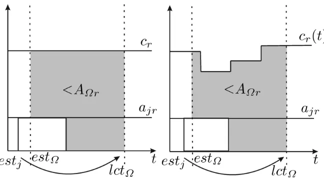
Extended Edge-Finding

Extended Edge-Finding rule was presented in [15]. It can be formulated as follows. Suppose that the taskj starts at estj, [estj, ectj) overlaps the interval [estΩ, lctΩ). Then if total amount of

resource required to process j and Ω in the interval [estΩ, lctΩ) is higher thancr(lctΩ−estΩ), then

Ω_lj holds, i.e. (Fig. 2 a)

(estΩ ∈[estj, ectj))∧(AΩr+ajr(ectj−estΩ)> Cr(lctΩ−estΩ))⇒Ωlj. (3)

Figure 2. Extended-Edge-Finding for a) constant resource capacity, b) piecewise constant resource capacity.

For generalized statement with capacity function cr(t) this rule can be written as (Fig. 2 b)

(estΩ ∈[estj, ectj))∧(AΩr+ajr(ectj −estΩ)> Z lctΩ

estΩ

cr(t)dt)⇒Ωlj. (4)

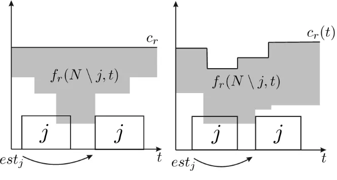
Time Tabling

Time Tabling rule ([7]) bases on calculation resource profile – an aggregation of compulsory parts [lstj, ectj) of tasks j ∈N which holds lstj < ectj

fr(Ω, t) =

X

j∈Ω|t∈[lstj,ectj)

Then the sweep technique of [3] is used to check resource overloads (Fig. 3 a)

(ectj > t)∧(cr < ajr+fr(N \j, t))⇒est0j > t.

The similar approach can be used to update lctj. This method was later improved in [14] and [4].

Figure 3. Time Tabling for a) constant resource capacity, b) piecewise constant resource capacity.

In terms of generalized statement this method can be written as (Fig. 3 b)

(ectj > t)∧(cr(t)< ajr+f(N \j, r, t))⇒est0j > t.

Note that if in the original algorithm we need to check overloads only in breakpoints of the function fr(N\j, t), which belong to the interval [estj, ectj). In this case, any breakpointt0 ∈[estj, ectj) of

the function Cr(t) is also have to be checked to get maximum domain propagation ofj ∈N.

Time Table Extended-Edge-Finding

Extended-Edge-Finding method was enhanced in [21] and [19] by combining it with Time Tabling. Let Af_Ωr – amount of resource r ∈R required to process tasks of the set Ω plus amount of resource used by compulsory parts of tasks of the set N \Ω over the interval [estΩ, lctΩ), i.e.

Af_Ωr=AΩr+

Z lctΩ

estΩ

f(N\Ω, r, t)dt.

Substituting AΩr byAf_Ωr in (1) and (3) gives Time-Table Extended-Edge-Finding rules.

This rules can be adopted for generalized statement by substituting AΩr byAfΩr in (2) and (4).

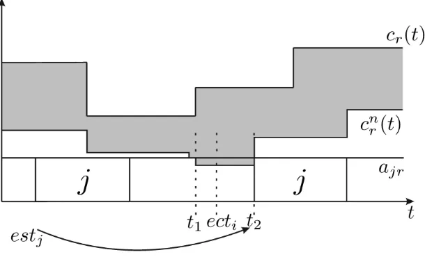
Strengthening Time-Table Edge-Finding

The following two rules can be used to make Time-Table Edge-Finding algorithm more efficient.

Figure 4. Strengthening Edge-Finding by consideringcn

r(t) on the interval [t1, t2) and a task i∈Ω.

1. Let us considercn

r(t) = cr(t)−fr(N, t) – the highest possible amount of resource which can

be used by non-compulsory parts of tasks. In section 4 we showed how to calculate this function. Edge-Finding rule can be enhanced by adding the following rules for set Ω ⊂ N and task j ∈N such that Ω_lj.

If for any t ∈ [t1, t2) such that [t1, t2) ∈ [estΩ, lctΩ)\[ectj, lstj) holds cnr(t)−ajr < 0 and

there is a taski∈Ω such that ecti ≥t1, then the earliest starting time of j can be updated:

est0_j :=t2 (Fig. 4).

2. Suppose there is a set Θ ⊆ Ω and moment of time t0 ∈ [estΘ, lctΘ)\[ectj, lstj), such that

cn_r(t0) < ajr holds. Then if amount of resource required to process non-compulsory parts of

all tasks of the set Θ is more then RlctΘ

estΘ cr(t)−ajrdt) and, then estj can be updated. I.e.

AΘr−

X

i∈Θ

air(|[lsti, ecti)∩[estΘ, t0)|)> Z t0

estΘ

(cr(t)−ajr)dt

then est0_j :=t0 (Fig 5).

This new rules can be combined with Time-Tabling Edge-Finding technique more powerful and give additional adjustments.

Capacity Function Adjustment

In the previous part, we showed how existing propagators can be adopted to generalized state-ment with resource capacity function and presented two new resource-based propagators. All mentioned propagators depend on the amount of resource available during the considered time in-terval. Therefore if we consider two instances of problem with the same sets of tasksN1 _≡N2 _with

Figure 5. Strengthening Edge-Finding by considering cn

r(t) and resource usage in [estΘ, t).

propagators is presented.

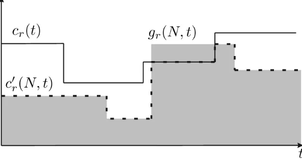
Figure 6. Capacity function adjustment.

Let us consider the following function

gr(Ω, t) =

X

j∈Ω|t∈[estj,lctj)

ajr. (5)

gr(N, t) represents an upper bound on amount of resource, which can be consumed by the tasks

of N at moment of time t. Therefore if for any t holds gr(N, t) < cr(t), then capacity function

cr(t) can be replaced byc0r(N, t) – thehighest possible consumption of resourcer ∈Rby the tasks

of the set N (Fig. 6). If cr(t) has a piecewise constant form with m breakpoints, the following

algorithm allows to calculate c0_r(N, t) in O(n+m) operations.

Algorithm 1. Highest possible consumption bounding.

Input: Set of tasksN,cr(t) with the set of breakpointsBPr.

Output: c0_r(N, t). 1: BPt=∅;

2: tsetgr(N, t) := 0;

3: for allj∈N do

4: ∀t∈[estj, lctj) increase gr(N, t)+ =ajr;

5: addestj andlctj toBPt;

6: end for

7: prevt= 0;

8: c0_r(N,0) = min{cr(0), gr(N,0)};

9: for allcurrentt∈BPr∪BPt\ {0} in increasing orderdo

10: ∀t∈[prevt, currentt) setc0r(N, t) := min{cr(prevt), gr(N, prevt)};

11: prevt:=currentt;

12: end for

13: Outputc0

r(N, t).

Note that this algorithm can be also applied to the classic statement with constant resource capacity. But as a result, the algorithm returns time-dependent piecewise constant highest pos-sible consumption of resource. Therefore the existing methods are not able to be applied to the considered problem statement and generalized Edge-Finding, Extended-Edge-Finding and Time Tabling methods can be applied to propagate task domains.

Project Makespan Estimation

All presented methods can be used in obtaining destructive project makespan lower bound defined by the following Theorem.

Theorem 1. If for any time horizon T after application of task domain and capacity function propagators one of the following conditions holds, there is no feasible schedule with makespan smaller or equal to T.

1. If for any j ∈N task domain [estj, lctj) will be not enough to process j, i.e. lctΩ−estΩ < P

j∈Ωpj.

2. Any set Ω⊆N does not have enough resource r∈R to process all tasks of Ω in its domain [estΩ, lctΩ) i.e.

RlctΩ

estΩ cr(t)dt < lctj−estj <

P

j∈Ω(ajrpj).

3. If for any resource r ∈ R and time moment t ∈ [0, T) amount of resource r ∈ R which can be used by non-compulsory parts of tasks is smaller than 0, i.e. cn

r(t)<0.

Using logarithmic search looking for the lowest possible time horizon T∗ for which all three statements of the Theorem 1 are incorrect, makespan lower bound T∗ can be obtained. Note that the search complexity and the quality of makespan lower bound depends on the considered sets Ω. If we consider Ω =i∈N, the search speed will be polynomial.

Conclusion

algorithm to clarify resource capacity function. These methods replenish the variety of constraint-programming techniques, which can be applied to RCPSP. We denote the function cn

r(t) which

represents an upper bound on the amount of resourcerwhich can be consumed by non-compulsory parts of tasks at timet, and presented an algorithm to calculate it in polynomial time. Well-known method of finding destructive makespan lower bound is replenished by the additional rule, based oncn_r(t) verification.

Acknowledgements

This research is supported by the Russian Foundation for Basic Research (grant 18-37-00295 mol a)

References

[1] P. Baptiste, C. Le Pape, and Nuijten W. Constraint-Based Scheduling. Kluwer Academic Publishers, 1998.

[2] N. Beldiceanu and M. Carlsson. Sweep as a generic pruning technique applied to the non-overlapping rectangles constraint. InProceedings of the 7th International Conference on Prin-ciples and Practice of Constraint Programming, pages 377–391, 2001.

[3] N. Beldiceanu and M. Carlsson. A new multi-resource cumulatives constraint with negative heights. In Proceedings of the 8th International Conference on Principles and Practice of Constraint Programming, pages 63–79, 2002.

[4] N. Beldiceanu, M. Carlsson, and E. Poder. New filtering for the cumulative constraint in the context of non-overlapping rectangles. In Proceedings of the 5th International Confer-ence on Integration of AI and OR Techniques in Constraint Programming for Combinatorial Optimization Problems, pages 21–35, 2008.

[5] J. Carlier and E. Pinson. An algorithm for solving the job-shop problem.Management Science, 35:164–176, 1989.

[6] Y. Caseau and F. Laburthe. Cumulative scheduling with task intervals. InProceedings of the Joint International Conference and Symposium on Lower bounds for Resource Constrained Project Scheduling Problem Logic Programming, pages 363–377. The MIT Press, Cambridge, 1996.

[7] B. R. Fox. Non-chronological scheduling. In Proceedings of AI, Simulation and Planning in High Autonomy Systems, pages 72–77, 1990.

[8] M. Garey and D. Johnson. Complexity results for multiprocessor scheduling under resource constraints. SIAM Journal on Computing, 4(4):397—-411, 1975.

[9] S. Gay, R. Hartert, and P. Schaus. Simple and scalable time-table filtering for the cumulative constraint. In Proceedings of the 21st International Principles and Practice of Constraint Programming CP, pages 149–157, 2015.

[10] B. Johnson. Efficient algorithms for shortest paths in sparse networks. Journal of the ACM, 24(1):1–13, 1977.

[11] R. Kameugne, L. Fotso, and J. Scott. A quadratic edge-finding filtering algorithm for cumu-lative resource constraints. InProceedings of the 17th International Conference on Principles and Practice of Constraint Programming CP, pages 478–492, 2011.

[12] A. Lahrichi. Ordonnancements. La notion de ”parties obligatoires” et son application aux problemes cumulatifs. RAIRO-Operations Research, 16:241–262, 1982.

[13] C. Le Pape. Des systemes d’ordonnancement flexibles et opportunistes. PhD thesis, Universite Paris XI, 1988.

[14] A. Letort, N. Beldiceanu, and M. Carlsson. A scalable sweep algorithm for the cumulative constraint. In Proceedings of the 18th International Conference on Principles and Practice of Constraint Programming, pages 439–454, 2012.

[15] L. Mercier and P. Van Hentenryck. Edge finding for cumulative scheduling.INFORMS Journal on Computing, 20(1):143–153, 2008.

[16] W. Nuijten. Time and resource constrained scheduling: A constraint satisfaction approach. PhD thesis, Eindhoven University of Technology, 1994.

[17] P. Ouellet and C. Quimper. Time-table extended-edge-finding for the cumulative constraint. In Proceedings of the 19th International Conference on Principles and Practice of Constraint Programming CP, pages 562–577, 2013.

[18] B. Roy and M. A. Sussman. Les problemes d’ordonnancement avec contraintes disjonctive. Tech. rep. Note DS 9, SEMA, Paris, 1964.

[19] A. Schutt, T. Feydy, and P.J. Stuckey. Explaining time-table-edge-finding propagation for the cumulative resource constraint. In Proceedings of the 10th International Conference on Integration of AI and OR Techniques and Constraint Programming for Combinatorial Opti-mization Problems, 2013.

[20] P. Vilim. Edge finding filtering algorithm for discrete cumulative resources in o(kn log n). In Proceedings of the 15th International Conference on Principles and Practice of Constraint Programming, pages 802–816, 2009.

[21] P. Vilim. Timetable edge finding filtering algorithm for discrete cumulative resources. In