https://itms-journals.rtu.lv
©2019 Oleg Uzhga-Rebrov, Ekaterina Karaseva, Vasily Karasev.
Computational Procedures of the Evidence Theory
for Interval and Fuzzy Assignments of the Basic
Probability Masses for Focal Elements
Oleg Uzhga-Rebrov
1, Ekaterina Karaseva
2, Vasily Karasev
3 1Rezekne Academy of Technologies, Rezekne, Latvia,
2
Saint-Petersburg State University of Aerospace Instrumentation, Saint-Petersburg, Russia,
3Institute of Problems of Mechanical Engineering of RAS, Saint-Petersburg, Russia
Abstract
–
The evidence theory is ascribed to a specific kind of uncertainty. In this theory, uncertainty refers to the fact that the element of our interest (the true world) may be included in subsets of other similar elements (possible worlds). In the original evidence theory, the estimates of the basic probability masses for the focal elements are given in an unambiguous form. In practice, to obtain such estimates is often difficult or even impossible. In such a situation, the relevant estimates are given in the interval or fuzzy form. The goal of the paper is to present and analyse the calculation procedures for determination of the belief functions and plausibility functions in the evidence theory for cases when the initial estimates are given in the interval or fuzzy form.Keywords – Belief function, data incompleteness, evidence theory, frame of discernment, focal elements, fuzzy value, inaccuracy, interval probability, interval value, membership function, plausibility function, probability mass, uncertainty.
I.INTRODUCTION TO THE EVIDENCE THEORY AND ITS EXTENSIONS
In this paper, we determine the ignorance as the situation where the necessary information is either missing, insufficient or presented in inappropriate form. In [1], the following forms of ignorance are highlighted: data incompleteness, inaccuracy
and uncertainty. According to this classification, the evidence theory is intended to process inaccurate and uncertain initial data.
For the first time, a rigorous scientific presentation of the evidence theory has been presented in [2]. Arthur P. Dempster in [3] proposed a specific version of the model with lower and upper probabilities and this work led to the further development of this theory.
The core concept of evidence theory is the frame of discernment
=
i/
i
=
1,..,
n
. The frame is formed byelements, which are interesting to us. The concept of elements can be interpreted very broadly, depending on the specific context. One of the elements of frame of discernment, which is true in the considered situation, is real, or true world, and is denoted as
0. Degrees of belief that the true world
0 belongs to certain subsets (focal elements) of the frame of discernment
, are assigned based on evidence. The function
: 2
0,1
m
→
is called the basic assignment of probabilitiesif
(1)
( ) 1
A
m A
=
for all A . (2)
The number m(A) is called the basic probability mass. If we have the basic assignments of probabilities for subsets
i
B
A
, then the overall degree of belief given to the subset (focal element)A
by m B( )
i ,B
i
A
is defined as(3)
A function
bel A
( )
: 2
→
0,1
is called the belief functionon
, if this function is given by (3) for some basic assignmentof probabilities
m
: 2
→
0,1
.The degree of plausibility for a focal element A is defined as
( )
1( )
pl A = −bel A . (4) The value pl(A) expresses the degree of extension where the subset A is plausible. The function
pl
: 2
→
0,1
is called the plausibility function. It is obvious that( )
1( )
bel A = − pl A (5) for all
A
.It follows that functions bel and pl are based on the same evidence and reflect the same state of knowledge.
The value pl(A) may be easily expressed in terms of the basic probability masses:
( ) 0,
m
=
( ) ( ).
i i B A
bel A m B
( )
( )
( )
( )
( )
1
.
i i
i
i i
B B A
i B A
pl A bel A m B m b
m B
= − = − =
=
(
6)Various methods for combining beliefs, derived from various sources, are proposed nowadays. These methods are not considered in this paper. A detailed summary of the most common methods is stated in [4].
The evidence theory in its original form supposes that the focal elements, based on the analysis, are given in a rigid deterministic form. Unfortunately, defining the relevant focal elements strictly is not always possible. There are many real-life examples where the focal elements can be defined either qualitatively or as linguistic categories for some variable. For the first time, L. Zadeh in his work [5] has indicated the potential possibility to extent the traditional evidence theory onto fuzzy focal elements. This extension was further developed in [6], [7].
In the original evidence theory, we assume that the values of the main probability masses for focal elements are given by a unique deterministic way. In other words, each basic probability mass is given by a single real number within the interval [0,1]. Often, by many reasons, setting such values is difficult or impossible. Some of these reasons are discussed in [8]:
- lack of analysis or assignment strategies (exact belief degrees may exist, but it can be difficult, or optional to extract them with high accuracy);
- instability (underlying beliefs may be unstable or the extraction of belief may be caused by extraction conditions);
- ambiguity (beliefs can be extracted through uncertain conclusions, such as “about 0.7”).
It follows that we should not always try to designate the exact values of the probability masses. It seems that, in uncertain initial situations, a more reasonable way is to introduce some degrees of uncertainty into the estimates of the relevant probability masses and, then, to make the necessary calculations based on these uncertain estimates.
There are two conceptual approaches to modelling the uncertainty of the values of the main probability masses: (1) specifying these values in the form of intervals; (2) specifying these values in the form of fuzzy numbers (linguistic categories). These approaches simulate different forms of expert’s ignorance regarding the estimated basic probability masses. Interval estimates indicate that the expert does not know the exact value of the estimated quantity, but he (she) is sure that the value is within the interval that he(she) sets. Fuzzy estimates correspond to the current expert’s knowledge about the actual value of the estimated variable (the value close to some fixed reference value).
II. THE CALCULATION OF THE INTERVAL VALUES bel{.} AND
pl{.} UNDER INTERVAL VALUES OF THE MAIN PROBABILITY MASSES
Let us make one important note before considering the basic concepts and definitions in this section and further. All further definitions and calculation expressions will be obtained under
the assumption of the presence of deterministic, uniquely defined focal elements on relevant analysis bases. However, all definitions and conclusions can be correctly applied to fuzzy focal elements.
Let us formulate the following problem: frame of discernment
is given; based on this frame of discernment, the set of focal elements is determined. For each of these elements, the basic probability mass is given as interval number,
i i i
m
=
m m
− +
, i=1,...,n. We need to calculate the interval values of the belief functions and plausibility functions for all focal elements.How can we calculate these interval values? Various approaches have been proposed to solve this problem. In [9], the author proposes calculating the boundary values of the
interval
( )
,( )
m m
bel− A bel+ A
by these expressions:
( )
max( )
,1( )
( )
;m
B A B A
bel− A m− B m+ B m+
= − −
(7)
( )
min( )
,1( )
( )
.m
B A B A
bel+ A m+ B m− B m−
= − −
(8)
Expressions (7) and (8) can be applied under the following condition: initial interval estimates of the basic probability masses are admissible. This means that the following conditions have to be true:
1
1
n
i i
m
−=
; (9)1
1
n
i i
m
+=
. (10)If conditions (9) and (10) are not true, the boundaries of the relevant intervals need to be corrected to satisfy these conditions. The correction determines the minimum and maximum limits of the intervals corresponding to the following expressions:
max ,1
i i j
j i
m− m− m+
=
−
, i=1,...,n; (11)min ,1
i i j
j i
m+ m+ m−
=
−
, i=1,...,n. (12)The calculated values
m
i−,m
i+ satisfy the following constraints:1
i j
j i
m
−m
+
−
, i=1,...,n; (13)1
i j
j i
m
+m
−
The basic probability masses, satisfying conditions (13) and (14), are called attainable interval probabilities. In any problem of calculation of the interval values of the belief and plausibility functions, the initial interval estimates of the basic probability masses should be admissible and attainable. Otherwise, correction of the initial data by expressions (11), (12) is required.
Let us consider a simple illustrative example. Frame of discernment
=
a b c
, ,
is given. On this frame, the following focal elements are allocated, which are assigned interval values of the basic probability masses:
a
with
,
0.1, 0.3
m
−a
m
+a
=
,
a b
,
with
,
,
,
0.2, 0.4
m
−a b
m
+a b
=
,
a c
,
with
,
,
,
0.3, 0.5
m
−a c
m
+a c
=
.We need to calculate the interval values of the belief function
. ,
.
m m
bel
−bel
+
for the given focal elements.First, we check the initial interval estimates by the attainability criteria (11), (12).
0.1 1(
,
,)
1(
0.4 0.5)
0.1;m− a = = − m+ a b +m+ a c = − + =
0.3 1(
,
,)
1(
0.2 0.3)
0.5 .m+ a = − m− a b +m− a c = − +
, 0.2 1(
,)
1(
0.3 0.5)
0.2 ;m− a b = = − m+ a +m+ a c = − + =
, 0.4 1(
,)
1(
0.1 0.3)
0.6 .m+ a b = − m− a +m− a c = − +
, 0.3 1(
,)
1(
0.3 0.4)
0.3 ;m− a c = = − m+ a +m+ a b = − + =
, 0.5 1(
,)
1(
0.1 0.2)
0.7 .m+ a c = − m− a +m− a b = − +
Obviously, the initial estimates of the basic probability masses are attainable interval estimates. Note, the attainability of interval estimates of the basic probability masses implies their admissibility but the opposite situation is not always true. Let us perform the required calculations by the expressions (7) and (8).
(
)
(
)
max
,1
,
,
max 0.1,1
0.4 0.5
max 0.1, 0.1
0.1
m
bel
−a
=
m
−a
−
m
+a b
+
m
+c
=
=
−
+
=
=
(
)
(
)
min
,1
,
,
min 0.3,1
0.2 0.3
min 0.3, 0.5
0.3
m
bel
+a
=
m
+a
−
m
−a b
+
m
−a c
=
=
−
+
=
=
(
)
(
)
,
min
,
,1
,
min
0.4 0.3 ,1 0.3
min 0.7, 0.7
0.7
m
bel
+a b
=
m
+a b
+
m
+a
−
m
−a c
=
=
+
−
=
=
(
)
(
)
, max , ,1 ,
max 0.3 0.1 ,1 0.4 max 0.4, 0.6 0.6
m
bel− a c = m− a c +m− a −m+ a b =
= + − = =
(
)
(
)
, min , ,1 ,
min 0.5 0.3 ,1 0.2 min 0.8, 0.8 0.8
m
bel+ a c = m+ a c +m+ a −m− a b =
= + − = =
The boundary values of the interval
plm−( )
A ,plm+( )
A
can be calculated as follows:
( )
max( )
,1( )
( )
;m
B A A B
pl− A m− B m+ B m+
=
= − −
(15)
( )
min( )
,1( )
( )
.m
B A A B
pl+ A m+ B m B− m−
=
=
−
− (16)Based on these expressions, we calculate the boundary values
.
pl
− ,pl
+
.
using the initial data from the example above.
max(
,
,)
,1( )
m
pl+ a = m− a +m− a b +m− a c −m+ =
(
)
max
0.1 0.2 0.3 ,1 0
max 0.6,1
1
=
+
+
−
=
=
.The specificity of this example is that the calculations of the
boundary values
pl
−
.
,pl
+
.
include estimates of the lower and upper limits of the main probability masses of all focal elements. This is due to the fact that the elementa
is included in all focal elements. To ensure the correctness of the calculations, we introduce zero probability mass, which is related to the empty set, according to expressions (15) and (16).
min(
,
,)
,1( )
m
pl+ a = m+ a +m+ a b +m+ a c −m− =
(
)
min 0.3 0.4 0.5 ,1 0 min 1.2,1 1
= + + − = = .
, max(
,
,)
,1( )
m
pl− a b = m a b− +m a− +m a c− −m+ =
(
)
max 0.2 0.1 0.3 ,1 0
max 0.6,1
1
=
+
+
− =
=
;
(
)
( )
, , ,
, min 1
m
m a b m a m a c
pl a b
m
+ + +
+
−
+ +
= =
−
(
)
min
0.4
0.3 0.5 ,1 0
max 1.2,1
1
=
+
+
−
=
=
.
(
)
( )
, , ,
, max 1
m
m a c m a m a b
pl a c
m
− − −
−
+
+ +
= =
−
(
)
(
)
, max , ,1 ,
max 0.2 0.1 ,1 0.5 max 0.3, 0.5 0.5
m
bel− a b = m− a b +m− a −m+ a c =
(
)
max 0.3 0.1 0.2 ,1 0 max 0.6,1 1
= + + − = = ;
, min(
,
,)
,1( )
m
pl+ a c = m+ a c +m+ a +m+ a b −m− =
(
)
min 0.5 0.3 0.4 ,1 0 min 1.2,1 1
= + + − = = .
For all focal elements, we get values
pl
m−
.
=
pl
m+
.
=
1.
This is a correct result associated with the specific assignment of the focal elements and the specific calculations by expressions (15) and (16).
In [10], [11], another approach for operations with interval values of the basic probability masses was proposed. We will not consider this approach, since the approach considered above seems to be more preferable because of simplicity and concreteness.
III. CALCULATION OF FUZZY VALUES
bel
m
.
ANDpl
m
.
UNDER FUZZY VALUES OF THE BASIC PROBABILITY MASSESThe fundamentals of the fuzzy set theory were published in [12]. A fuzzy number is a fuzzy set defined on a set of real numbers. Let us suppose that, due to the lack of expert knowledge, the main probability masses for focal elements are presented in the form of triangular fuzzy numbers.
How can fuzzy values
bel
m
.
,pl
m
.
be calculated? To do it, the
-cuts at the levels of our interest are determined on the graphs of the membership functions of the relevant fuzzyvalues
m
i
.
. Thus, at each level
we have a set of interval values of the relevant probability masses. Interval values of thefunction
bel
m−
. ,
bel
m+
can be calculated by expressions (11), (12). Combining the obtained intervals, we can consider agraph of the membership function of a fuzzy number
bel
m
.
. Similarly, interval values
pl
m−
. ,
pl
m+
.
can be calculated at given
-levels, using expressions (15) and (16). Combining the obtained interval values, we can construct agraph of the membership function of a fuzzy number
pl
m
.
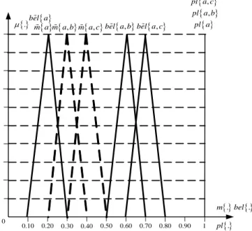
. Let us take as a basis the initial interval values of the main probability masses from the example presented above. On these intervals, as on the bases, let us form the following symmetric triangular fuzzy numbers m a (
= 0.1, 0.2, 0.3)
,
, 0.2,0.3,0.4
m a b = , m a c
(
, = 0.3, 0.4, 0.5)
. Graphs of the membership functions of these fuzzy numbers are shown in Fig. 1.Let us define the
-levels with increment 0.1. Thepreviously calculated intervals of values
bel
m−
. ,
bel
m+
.
are the bases for the desired fuzzy numbers. Performing calculations for all given
-levels and combining the obtainedintervals, we obtain the desired fuzzy numbers
bel
m
.
; the graphs of their membership functions are shown in Fig. 1.Calculation of fuzzy estimates
pl
.
is made by analogy, using expressions (15) and (16).Fig. 1. Graphs of the membership functions of the initial fuzzy values m
.and final fuzzy estimates bel
. and pl
. in an illustrative example. In the present example, the estimatespl
.
remain deterministic and equal to 1 at all
-levels. Let us note again that such values are associated with specific focal elements and specific estimates of the main probability masses in the considered example only.IV. CONCLUSION
The evidence theory has been developed to handle a specific type of uncertainty: the entity of interest can be in subsets (focal elements) of a universal set (a basis of analysis). The degree of certainty that a given entity is located in a concrete focal element is evaluated by the value of the basic probability mass given to this focal element. Derived estimations of belief degrees and plausibility for interacting focal elements are performed with special expressions based on estimations of the main probability masses for the relevant initial focal elements.
The original evidence theory assumes: the initial focal elements and estimations of the probability masses, given to these focal elements, are given in deterministic form. However, in practice, often we cannot obtain deterministic values of the basic probability masses. To solve this problem, the initial estimations of the basic probability masses can be given in a suitable undetermined form.
This paper presents computational procedures for determination of the values of belief and plausibility functions in extended versions of evidence theory when estimates of the basic probability masses are given either as intervals or as fuzzy numbers. The emergence of such extensions of the original evidence theory is associated with the requirement to operate with indefinite estimates, which are caused by the lack of
0.10 0
0.20 0.30 0.40 0.50 0.60 0.70 0.80 0.90 1
.
bel am a m a b , m a c , bel a b , bel a c , pl a
,
pl a b
,
pl a c
.
m bel.
.
knowledge among experts regarding the analysed uncertain situations.
In the paper, we have used an approach to the determination of the interval values of the functions
bel
.
andpl
.
proposed in [9]. An alternative approach is described in [10], [11]. To our mind, the considered approach is preferable.Analysing the research presented in the paper, we can draw an undoubted conclusion: the interval extension of the original evidence theory is decisive. The basis of the fuzzy extension of this theory is the interval extension.
In recent decades, various approaches have intensively been developed, which allow us to successfully process various types of uncertain initial data. The extensions of the evidence theory presented in this paper confirm this trend.
REFERENCES
[1] N. Burrus, D. Lesage, “Theory of Evidence”, Laboratorie de Reserche et Développment de lʹEpita, France, Tech. Rep., 2011.
[2] G. Shafer, A mathematical theory of evidence. Princeton University Press, 297 p., 1976.
[3] P. Dempster, “Upper and lower probabilities induced by a multivalued mapping”, Annals of Mathematical Statistics, vol. 38, no. 2, pp. 325–339, 1967. https://doi.org/10.1214/aoms/1177698950
[4] O. Uzhga-Rebrov, Uncertainties management. Part 3. Modern non-probabilistic methods. Rezekne, RA Izdevniecība, 560 p., 2010. (In Russian).
[5] L. Zadeh, “Fuzzy sets and information granularity”, in Advances in Fuzzy Sets Theory and Applications, R. K. Ragade, M. M. Gupta, and R. R. Yager (editors). 1979, pp. 3–18.
[6] J. Yen, “Generalizing the Dempster-Shafer Theory to Fuzzy Sets”, IEEE Transactions on Systems, Man and Cybernetics, vol. 20, no. 3, pp. 559–570, 1990. https://doi.org/10.1109/21.57269
[7] M.-Sh. Yang, T.-Ch. Chen, K.-L. Wu, “Generalized Belief Function, Plausibility Function, and Dempster’s Combinational Rule to Fuzzy Sets”, International Journal of Intelligent Systems, vol. 18, no. 8, pp. 925–937, 2003. https://doi.org/10.1002/int.10126
[8] P. Walley, Statistical Reasoning with Imprecise Probabilities. Chapman and Hall, London, etc., 706 p., 1991.
[9] T. Denoeux, “Reasoning with imprecise belief structures”, International Journal of Approximate Reasoning, vol. 20, no. 1, pp. 79–111, 1999.
https://doi.org/10.1016/S0888-613X(98)10023-3
[10] K. Weichselberger, “The Theory of Interval-Probability as a Unifying Concept for Uncertainty”, International Journal of Approximate Reasoning, vol. 24, no. 2–3, pp. 149–170, May 2000.
https://doi.org/10.1016/S0888-613X(00)00032-3
[11] K. Weichselberger, Th. Augustin, “On the Symbiosis of Two Concepts of Conditional Interval Probability”, in ISIPTA’03, J. Bernard, T. Seidenfeld, and M. Zaffalon (Editors), Waterloo, Carleton Scientific, 2003, pp. 608–630.
[12] L. Zadeh, “Fuzzy Sets”, Information and Control, vol. 8, no. 3, pp. 338–353, 1965. https://doi.org/10.1016/S0019-9958(65)90241-X
Oleg Uzhga-Rebrov is a Chief Researcher of the Information and
Communication Research Institute at Rezekne Academy of Technologies (Latvia). He received his Doctoral degree in Information Systems from Riga Technical University in 1994. He has 81 scientific works, including 5 monographs. He is an expert of the Scientific Council of Latvia. His research interests include different approaches to processing incomplete, uncertain and fuzzy information, in particular, fuzzy set theory, probabilistic inference, fuzzy inference, decision analysis and risk analysis.
E-mail: [email protected]
Ekaterina Karaseva is an Associate Professor of the Department of
Entrepreneurial Information Technologies, Saint-Petersburg State University of Aerospace Instrumentation (Russia). She received her qualification (economist) from the Belorussian State University of Economics, Faculty of Banking and Finance in 2007 (Belarus Republic). She has also a degree of Candidate of Economic Science (2013), the Doctoral Thesis entitled “Estimate and Regulation of Operational Risk in Bank”. Her research interests include operational risk, financial risk, banking and modelling, system analysis and decision-making procedures.
E-mail: [email protected]
ORCID iD: https://orcid.org/0000-0002-3286-0959
Vasily Karasev is a Senior Researcher of the Automated Design Laboratory of
Intelligent Integrated Systems, Institute of Problems of Mechanical Engineering of the Russian Academy of Sciences (Russia). He is a candidate of technical science (2000). His research interests include logic, probability theory, combinatorial analysis, optimisation methods, graph theory, classification methods, expert systems, system analysis and artificial intelligence technologies.