Slow magnetoacoustic waves in coronal loops : EIT and TRACE

University of Warwick institutional repository: http://go.warwick.ac.uk/wrap

This paper is made available online in accordance with

publisher policies. Please scroll down to view the document

itself. Please refer to the repository record for this item and our

policy information available from the repository home page for

further information.

To see the final version of this paper please visit the publisher’s website.

Access to the published version may require a subscription.

Author(s): E. Robbrecht, E. Verwichte, D. Berghmans, J. F.

Hochedez, S. Poedts, V. M. Nakariakov

Article Title: Slow magnetoacoustic waves in coronal loops: EIT and

TRACE

Year of publication: 2001

Link to published article:

http://dx.doi.org/10.1051/0004-6361:20010226

DOI: 10.1051/0004-6361:20010226 c

ESO 2001

_Astrophysics

&

Slow magnetoacoustic waves in coronal loops: EIT and TRACE

E. Robbrecht1,2, E. Verwichte2, D. Berghmans2, J. F. Hochedez2, S. Poedts1,?, and V. M. Nakariakov3

1

Centre for Plasma Astrophysics, K.U. Leuven, Celestijnenlaan 200B, 3001 Leuven, Belgium 2 _{Royal Observatory of Belgium, Ringlaan 3, 1180 Brussel, Belgium}

3

Physics Department, University of Warwick, Coventry CV4 7AL, UK

Received 20 November 2000 / Accepted 6 February 2001

Abstract. On May 13, 1998 the EIT (Extreme ultraviolet Imaging Telescope) on board of SoHO (Solar and Heliospheric Observatory) and TRACE (Transition Region And Coronal Explorer) instruments produced simul-taneous high cadence image sequences of the same active region (AR 8218). TRACE achieved a 25 s cadence in the Feix _{(171 ˚A) bandpass while EIT achieved a 15 s cadence (operating in “shutterless mode”, SoHO JOP 80)}

in the Fexii(195 ˚A) bandpass. These high cadence observations in two complementary wavelengths have revealed

the existence of weak transient disturbances in an extended coronal loop system. These propagating disturbances (PDs) seem to be a common phenomenon in this part of the active region. The disturbances originate from small scale brightenings at the footpoints of the loops and propagate along the loops. The projected propagation speeds roughly vary between 65 and 150 km s−1 _{for both instruments which is close to and below the expected sound} speed in the coronal loops. The measured slow magnetoacoustic propagation speeds seem to suggest that the transients are sound (or slow) wave disturbances. This work differs from previous studies in the sense that it is based on a multi-wavelength observation of an entire loop bundle at high cadence by two EUV imagers. The observation of sound waves along the same path shows that they propagate along the same loop, suggesting that loops contain sharp temperature gradients and consist of either concentric shells or thin loop threads, at different temperatures.

Key words.Sun: activity – Sun: corona – Sun: oscillations – Sun: UV radiation – MHD – waves

1. Introduction

In this paper we report on the detection and study of propagating disturbances (PDs) along coronal loops.

Our study is focused on active region AR8218, us-ing image sequences of JOP80 (Clette et al. 1998). This JOP (Joint Operation Project) was performed on May 13, 1998 and produced simultaneously high cadence image se-quences of the same active region in different wavelengths. The analysis in this paper is based on observations of two instruments measuring in two different wavelengths: EIT (Extreme ultraviolet Imaging Telescope) on board SoHO (Solar and Heliospherical Observatory) measures in 195 ˚A and TRACE (Transition Region And Coronal Explorer) measures in 171 ˚A. A previous study on the EIT data has been done by Robbrecht et al. (1999) in which they dis-cuss the detection of PDs in coronal loops. They show that slow magnetoacoustic waves are a possible interpretation of these PDs. In the present paper we find stronger evi-dence for this hypothesis, based on a study of the TRACE

Send offprint requests to: E. Verwichte, e-mail:[email protected]

? _{Research Associate of the Fund for Scientific Research in} Flanders (FWO-Vlaanderen).

data (part of JOP80) and the comparison between the TRACE and the EIT data.

There exist many observations of time variability in active region loops. Aschwanden et al. (1999) give a very broad overview of spatial oscillations of coronal loops and coronal loop dynamics in general. Svestka et al. (1982a, 1982b) observed quasi-periodic brightness varia-tions. Roberts et al. (1984) suggested that these quasi-periodic variations might be caused by free, slow-mode MHD (Magneto-HydroDynamic) oscillations of large scale loops. Later they observed phenomena they called “flar-ing arches”: propagat“flar-ing brighten“flar-ings seen in X-rays and streaming material in Hα in a giant arch preceded by a flare (Martin & Svestka 1988; Svestka et al. 1989). Harrison (1987) observed for the first time soft X-ray pul-sations from the non-flaring Sun. The pulpul-sations originate from a compact active region which lies at one footpoint of a large coronal loop. The periodicity is thought to be produced by a standing wave or a traveling wave “packet” which exists within the loops. With the recent operation of more powerful instruments, the list of observational ev-idence for variability in coronal loops is largely extended. Brekke et al. (1997) reported of the first observations of high-velocity flows in active region loop systems ob-served with the CDS (Coronal Diagnostic Spectrometer)

on SoHO. The velocities observed at a temperature of 240 000 K are of the order of 50–60 km s−1_{. They find,}

within the same loop system, velocities in opposite direc-tions seen in neighbouring loops. They argue these dis-turbances are not caused by mass-flows along the loops because that would require velocity values considerably larger than the measured values. Kjeldseth-Moe & Brekke (1998) investigated loops at temperatures ranging from 104 _{K to 2.7 10}6_{K using CDS. By investigating Doppler}

line shifts, velocities from 20 km s−1 _{up to 300 km s}−1

have been found. They mention magnetoacoustic waves as a possible explanation of the line shifts. Berghmans & Clette (1999) first discussed a new class of weaker foot-point brightenings that produce wave-like disturbances propagating along quasi-open field lines, which have been further analyzed by Robbrecht et al. (1999) and which will also be studied in this report. Also more recently De Moortel et al. (2000) reported on similar propagating oscillations in large diffuse coronal loops, using TRACE data. Not only longitudinal oscillations, but also trans-verse oscillations of active region loops have been observed directly (e.g. Aschwanden et al. 1999; Nakariakov et al. 1999).

The phenomenon of propagating disturbances along loops is comparable to moving features observed in po-lar plumes. DeForest & Gurman (1998) reported on the observation of outward propagating features in plumes, traveling outward at speeds of 75–150 km s−1 along the plume structure. They argued that these moving features are slow magnetoacoustic waves because

1. the propagation speed is always less than the sound speed of the observation;

2. the moving features repeat in quasi-periodic trains; and

3. Doppler shifts have not been reported in plumes for these speeds.

Ofman et al. (1999) reported on an increase in rela-tive intensity of the features with radial distance and found a good match between the observations and a one-dimensional analytical model of spherical slow magnetoa-coustic waves in a stratified atmosphere.

Nightingale et al. (1999) have analyzed the time vari-ability of EUV brightenings in coronal loops, based on TRACE data in the 171 ˚A line. They conclude that these small EUV (Extreme UltraViolet) brightenings cannot be associated with upflows of heated plasma by chromo-spheric evaporation, consequently they also do not con-tribute to coronal heating. Instead, their near-isothermal density enhancements seem to be caused by compressional waves, which start near the loop footpoints and propagate along the loops with approximate sound speed.

Contrary to the acoustic wave interpretation, Reale et al. (2000) interpreted the evolution of a transient bright-ening of a coronal loop, observed by TRACE, in terms of an initially empty and cool magnetic flux tube along which plasma motion takes place. This interpretation is inspired by a transient heating episode occurring along

the loop. However, Nakariakov et al. (2000) have shown that the propagating disturbances in coronal loops can be interpreted as slow magnetoacoustic waves analogously to waves in coronal holes.

The studies mentioned above are all important in the process of understanding the heating and dynamics of coronal loops. However, up to now an important factor was missing: the ability of comparing observations in dif-ferent wavelengths. This is a powerful tool since it can be used, not only to observe coronal features instantaneously at different temperatures, but also to check measured val-ues (propagation speeds, inclination angles of loops with respect to the field of view and their interpretation. The importance of this paper lies in this crucial factor of simul-taneously observing the same coronal feature at different wavelengths.

In Sect. 2 the data sets and the morphology of the active region are described. Section 3 contains an expla-nation of the analysis, leading to the slow magnetoacoustic wave interpretation. The results are described in Sect. 4 which are followed by a discussion.

2. Observations

On May 13, 1998, the EIT instrument on board SoHO and TRACE telescope have produced a unique image se-quence in the context of the multi-instrument campaign SoHO JOP80 (Clette et al. 1998). JOP80 is dedicated to the high-time resolution imaging study of coronal and transition region dynamics (EIT shutterless-mode cam-paign). The initial aim was to study bright structures (active region loops, bright points) with the highest pos-sible time resolution and wide spatial coverage. First re-sults of this JOP80 have been reported by Berghmans & Clette (1999); Robbrecht et al. (1999). In JOP80, EIT is the lead instrument, followed by several space-born in-struments: SXT (Soft X-ray Telescope), TRACE, MDI (Michelson Doppler Imager), CDS (Coronal Diagnostics Spectrometer), SUMER (Solar Ultraviolet Measurements of Emitted Radiation), as well as two ground based obser-vatories (in La Palma and Sac Peak). The combination of these instruments allows for good statistics of many local events.

2.1. EIT data

EIT (Extreme ultraviolet Imaging Telescope, Delaboudini`ere et al. 1995; Tarbell 1994) achieved an exceptional 15 s cadence in the Fexii bandpass

Table 1. Characteristics of the JOP80 dataset produced by the EIT and TRACE instruments. The bandpasses of EIT Fe XII (195 A) and TRACE Fe IX (171 A) are narrow with a peak formation temperature of respectively 1.6 MK and 1 MK. The end time of the TRACE sequence is determined by cosmic rays which damaged the images too much

Instrument EIT TRACE

Bandpass 195 ˚A 171 ˚A

Ion Fexii Feix

Level Corona Low Corona

Temp 1.6 MK 1 MK

Cadence 15 s 25 s

Pixelsize 2.59 arcsec/pix 0.5 arcsec/pix starttime 17h 31m 50s 17h 03m 28s

endtime 18h 29m 07s 18h 07m 17s

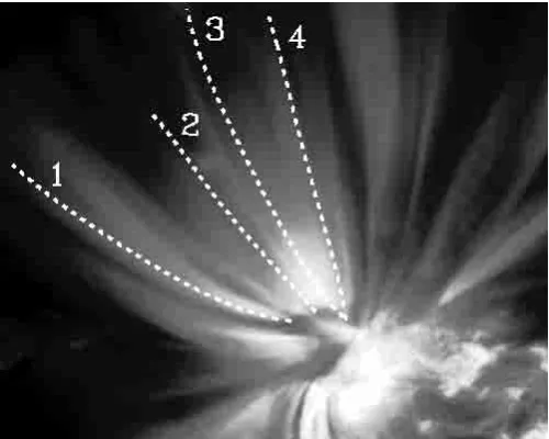
Fig. 1.The field of view of EIT, specified in the full disc in

Fig. 3. Superimposed we have drawn the field of view of the TRACE image which is shown in Fig. 2

that appear in one image only. Their values were restored by replacing the pixel’s intensity with a linear interpola-tion from neighbouring images. See Delaboudini`ere et al. (1995) and Berghmans & Clette (1999) for more technical details. Due to the solar rotation, the active region shifts to the right of the field of view during the 1 hour observation campaign by less than 4 EIT pixels. This shift was compensated to a subpixel level by determining the maximum of cross-correlation between the images.

2.2. TRACE data

The TRACE (Transition Region And Coronal Explorer, Handy et al. 1999) dataset consists of a datacube with a spatial size of 1024×1024 pixels and a temporal sequence of 147 images at a cadence of 26 s in the Feix_bandpass

(171 ˚A). The image sequence starts at 17:03:28 UT and

Fig. 2. The field of view of TRACE, specified in Fig. 1. In

Figs. 5 to 8 we give the characteristics of the 4 loops tracked here

ends at 18:07:17 UT on 1998 May 13, with a total du-ration of 3829 s. A subregion of 400×355 pixels (200× 177.5 arcsec) has been selected from the whole field of view. There is not a complete match (spatially and tem-porally) between the EIT and the TRACE datasets (see Fig. 1 and Table 1 resp. for the spatial and temporal align-ment). Due to cosmic rays, the last part of the TRACE sequence cannot be used and therefore there is only half an hour overlap between the two data sets. To clean the TRACE data we used standard procedures found in the SolarSoft TRACE analysis guide (?). The TRACE im-ages suffer greatly from radiation noise spikes due to the radiation belt passages. In the time period between 17h28 and 17h35 the cosmics are severe. The pixels hit by cosmic rays (exceeding the 6σlevel) are replaced by a nearby pixel value. We removed the background diffraction pattern by applying a Fourier analysis on the data. The TRACE im-ages were corrected for solar rotation and spacecraft jitter by determining the shift for maximum cross-correlation between the images. The internally co-aligned EIT and TRACE data cubes were then mutually co-aligned on the basis of the image headers pointing information. An improvement on this was achieved by visually identify-ing a relative large number (>10) of distinctive features that could be recognized in both images. An optimal co-ordinate transformation is then constructed (least mean square basis) that maps the TRACE image to the EIT image and vice versa. All this results in an EIT-TRACE co-alignment better than 1-2 EIT pixels which is sufficient for the present study.

2.3. Active region 8218

Fig. 3.At the left, an EIT full disc image in the Fexii(195 ˚A)

bandpass, taken at 18h 34m UT. The rectangle indicates the active region AR 8218, it corresponds to the EIT field of view.

At the right, a side view on AR 8218 when crossing the western limb. This image has been processed to enhance the edges of the loop structure

variety of transients was discovered, ranging from a B3.5 flare producing a large plasma flow along pre-existing loops, to EUV versions of active region transient brighten-ings as previously observed by SXT on board YOHKOH (Berghmans & Clette 1999; Shimojo 1998). In Fig. 3 (left), we show the overall structure of this active region and fo-cus (Fig. 1) on the bundle of long, magnetic flux tubes that emanates from it to the NE. The width of the EIT field of view is about 2.3 108 _{m (0.34R}

). Taking profit

of the solar rotation and assuming that the overall struc-ture of this bundle remained unchanged over a period of a week, we obtained a side view of the active region when it crossed the western limb (Fig. 3,right). From this we estimate that the magnetic flux tubes in the bundle make an angle α with the plane of the sky that ranges from roughly 30◦ up to 70◦.

3. Investigating the loops

Here we focus on an additional, new type of transients that was discovered propagating along the bundle of widely opening magnetic field lines in the NE of the active re-gion. In this region, loops are quite clear. To illustrate the variability of the analyzed loop system we show in Fig. 4 a sequence of 4 running difference images at 171 ˚A, and 195 ˚A. Dark and bright features, outlining the whole length of a loop, suggest that the loops also experience transverse motions. The pattern of diagonal lines in the TRACE sequence of difference images is an instrumental artifact. They are remains of the background diffraction pattern, which are enhanced by the differencing. In a dif-ference movie, we see a continuous outflow of bright dis-turbances. After a sudden brightening at the footpoint of the fan of loops we detect a quasi-periodical radial outflow of disturbances, along the loops. Figure 4 illustrates the propagation of a PD by making running difference images. The PDs are indicated with a white arrow. Note, that the

Fig. 4.Two sequences of 4 “running time difference” images

are shown, extracted from TRACE 171 ˚A, images (at the left) and from EIT 195 ˚A, images (at the right). The difference im-ages are created by subtracting an image taken 2m 15s (for TRACE) and 1m 54s (for EIT) earlier than the time men-tioned in the upper left corner. We notice that there is no correspondence between the time of TRACE and EIT. White arrows indicate the propagation of a disturbance

sequences of TRACE and EIT do not correspond in time here.

the two instruments. We then applied a transformation to obtain the same path in the EIT data. The transformation method is described in Sect. 2.2. The width of the path is equal to the pixelsize of the instrument. The path in the EIT data is generally shorter, since the field of view is smaller at the North of the active region, where the loops are tracked. By assuming a semi-circular loop, we visually estimate the length along an entire loop to be 800 Mm. The path length (projection onto the field of view) is es-timated to be of the order of 100 Mm.

3.1. Slow magnetoacoustic wave interpretation

In Figs. 5 to 8 we show the temporal evolution (hori-zontal axis) along the four selected paths (vertical axis). A quadratic fit to each pixel’s light curve was calculated. This quadratic fit is taken as the slowly varying, EUV emission background. The relative variations with respect to this background is shown. In this diagram we see prop-agating disturbances as bright and dark diagonal ridges. From this diagram, the apparent propagation speedvpof

each disturbance along the loop is deduced, by measuring the slope of its respective ridge. This is done by hand. The speed we measure is apparent because we only measure the component projected onto the plane of the sky. Here the interpretation of slow magnetoacoustic waves makes its way. EIT (1.6 MK) measures at a higher temperature than TRACE (1 MK). The sound speed CS can be

ex-pressed in function of temperature alone (Priest 1984). This allows us to derive a formal sound speed:

CS = 152 T1/2m s−1(T in K),

= 152 km s−1 for TRACE data (171 ˚A), (1) = 192 km s−1 for EIT data (195 ˚A). (2) The expected sound speed is higher for the EIT obser-vations than for the TRACE obserobser-vations (see Table 1). The apparent propagation speedsvp which we list in the

four tables, are of the order of, but never exceed this de-rived sound speed. This suggests that these PDs are sonic perturbations.

If we assume this, then the difference between the mea-sured speed and the sound speed is explained by the pro-jection onto the plane of the sky. This means that we can derive from the difference between the apparent speed and the sound speed, the projection angle αexp between the

loop direction and the plane of the sky:

αexp= arccos

vp

CS

· (3)

3.2. Discussion of measurements

For each of the four paths we have plotted the time-space diagram for TRACE and EIT, in such a way that the times correspond vertically (Figs. 5 to 8). The letters under the diagrams indicate the starting points of the PDs of which we measured the apparent speed. These letters are written

in the tables in the column labeled “l”. In some cases, a particular disturbance occurs in the two data sets, such that comparison between the two data sets is possible. The tables describe the measured speeds quite in detail.

vpis the apparent speed. We measured this speed for each

ridge at the bottom of the path (<20 Mm starting from the footpoint of the loop which is not the same as the starting point of the path), at the top (>20 Mm) and over the full length of the path. The error is calculated ass.e.=√σ2_n

where σ2 is the variance and n the number of measure-ments of the slope of the PD in the diagram. With each speed, there is a corresponding projection angleαexp. This

is calculated through formula (3). In the tables we list the interval [αexp(vp−s.e.), αexp(vp+s.e.)]. If this interval lies

entirely in the interval [30◦,70◦], for both datasets, then our measurements do not speak against the slow magne-toacoustic wave interpretation.

We now briefly describe the four paths in detail. To simplify the description, we will use the following notation: “Tb” means PD b in the TRACE dataset, “Ea” is PD a in the EIT dataset.

3.2.1. Path 1

The footpoint of the loop lies at roughly 10 Mm above the starting point of path 1. In each diagram we can dis-tinct a broad bright ridges, Tc and Ec. They have an ap-parent speed of respectively 105 and 124 km s−1. The projection angles lie in the ranges [40◦,52◦] and [45◦,54◦] resp. Both intervals are acceptable (i.e. lie between 30◦ and 70◦). Moreover, there is a broad overlap between the two intervals ([45◦,52◦]), which indicates that we can be sure to measure PDs in the same loop. Assuming that Tc and Ec have the same physical origin, we could measure a period of 30 min between these two PDs. Furthermore there are thinner PDs with roughly the same speed as in Tc and Ec, apart from PD Td, which propagates at a re-markably lower speed. Nevertheless, the angle deduced for PD Td is still acceptable.

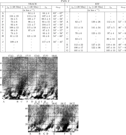
3.2.2. Path 2

The footpoint of the loop lies at roughly 10 Mm above the starting point of path 2. Remark that the EIT frame was to small to contain the whole path. An overall clear diagonal structure is visible in both diagrams. The average (weighted) propagation speed in the TRACE frame is 95± 1 km s−1_{inferring an expected angle ofα}

exp= 51±1◦and

111± 3 km s−1 _{in the EIT frame, inferring an expected}

angle of αexp = 55±1◦. In calculating the average speed

Path 1

TRACE EIT

l vp(<20 Mm) vp(>20 Mm) vp αexp l vp (<20 Mm) vp(>20 Mm) vp αexp

(in km s−1_{) (in km s}−1₎

A 71±12 121±13 88±8 50◦−58◦ - - -

-B 74±6 100±25 88±5 52◦−57◦ - - -

-C 114±8 105±11 40◦−52◦ - - -

-D 64±11 75±21 50◦−70◦ A 125±8 121±21 134±11 41◦−50◦

E 74±11 119±23 94±12 46◦−57◦ - - -

-F 104±20 126±27 119±11 31◦−45◦ - - -

-- - - - B 129±29 128±24 126±14 43◦−54◦

- - - - C 151±23 118±16 124±12 45◦−54◦

- - - - D 113±24 126±13 43◦−54◦

- - - - E 116±10 124±10 45◦−54◦

Fig. 5.The EUV intensity along path 1 as a function of time (horizontal axis) and distance along the path (vertical axis) in

the TRACE data (upper) and in the EIT data (lower) tracked in Fig. 2

respect to the other PDs. PD Ti does not reach as high, therefore its total speed will be more dominated by lower height. In the TRACE frame starting at 17:28 at height 20 Mm we can measure a period of 5 min between the PDs. In EIT we only seem to measure a period of 10 min. There is a good overlap of measurements: Tf and Ea; Te and Eb; Ti and Ec. The expected projection angles match well. PDs Ec and Ed seem to be of a different population. Perhaps two loops are contained in the path. If we exclude Ec and Ed we find an average speed 120±4 km s−1giving an angle of αexp = 50±1◦ good corresponding to the

average angle deduced from the TRACE data.

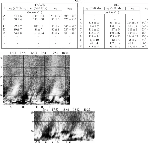
3.2.3. Path 3

Path 2

TRACE EIT

l vp (<20 Mm) vp(>20 Mm) vp αexp l vp (<20 Mm) vp (>20 Mm) vp αexp

(in km s−1_{) (in km s}−1₎

A - 64±4 64±4 63◦−67◦ - - - -

-B 124±19 113±14 107±4 43◦−47◦ - - - -

-C 84±5 105±7 88.5±3 53◦−56◦ - - - -

-F 73±6 96±4 93±15 44◦−59◦ A 62±7 139±26 112±6 52◦−57◦

D 93±8 111±7 104±5 44◦−50◦ - - - -

-E 100±13 115±18 102±4 46◦−50◦ B 111±14 141±34 127±5 46◦−51◦

G 68±9 97±8 87±5 53◦−57◦ - - - -

-I 74±3 - 83±3 58◦−56◦ C 70±6 123±13 97±4 58◦−61◦

H 81±13 121±18 83±6 54◦−60◦ - - - -

-- - - D 63±5 - 80±14 61◦−70◦

J 109±8 - 117±9 34◦−45◦ - - - -

-- - - E 112±22 127±21 110±16 49◦−61◦

- - - F 100±17 122±36 107±14 51◦−61◦

- - - G 101±11 - 105±13 52◦−61◦

Fig. 6.The EUV intensity along path 2 as a function of time (horizontal axis) and distance along the path (vertical axis) in

the TRACE data (upper) and in the EIT data (lower) tracked in Fig. 2

repetition of PD Ta. If this would be the case, we would measure a period of about 30 min, which we also have found in Path 1. As mentioned in the table, there are two other pairs of matching PDs being Tc and Eb, and Td and Ec.

3.2.4. Path 4

The footpoint is at about 10 Mm of the starting point of the path. It is difficult to find similarities between the

Path 3

TRACE EIT

l vp (<20 Mm) vp (>20 Mm) vp αexp l vp (<20 Mm) vp (>20 Mm) vp αexp

(in km s−1_{) (in km s}−1₎

A 54±5 114±14 87±12 49◦−61◦ - - - -

-B 58±4 111±10 86±6 52◦−58◦ - - - -

-- - - A 124±11 137±19 124±13 44◦−55◦

C 92±7 105±5 86±2 54◦−57◦ B 104±7 106±12 106±7 54◦−59◦ D 89±7 88±7 86±8 52◦−59◦ C 111±12 137±5 112±3 53◦−56◦ E 83±8 107±13 93±7 48◦−56◦ D 118±14 139±27 126±9 45◦−53◦

- - - E 129±24 155±20 124±12 45◦−54◦

- - - F 59±10 112±4 79±3 64◦−67◦

- - - G 46±4 102±12 70±10 65◦−72◦

- - - H 114±11 131±10 120±7 48◦−54◦

Fig. 7.The EUV intensity along path 3 as a function of time (horizontal axis) and distance along the path (vertical axis) in

the TRACE data (upper) and in the EIT data (lower) tracked in Fig. 2

3.3. Variability

In order to quantify the variability in the loops, we define two different parameters for each pixel (x, y):

1. σa(x, y): the standard deviation with respect to the

median image, expressed in DN. This quantity is a measure of the combined effect of various tempo-ral variability components, such as slow background trends, rapid transients and oscillatory fluctuations, but also random variations due to instrumental noise; 2. σn(x, y): the expected instrumental noise level also

ex-pressed in DN. The main contributions to the instru-mental noise are the photon shot noise (Poisson statis-tics), here calculated as a function of intensityI, and

the CCD readout noise:

σn = √0.25I+ 2.7, for EIT (195 ˚A);

= √0.08I+ 2.8, for TRACE (171 ˚A); (4) with I the observed intensity expressed in DN. At times of cosmic snow, the noise from cosmic-ray re-moval dominates. This occurs mainly in the TRACE data between 17:28 UT and 17:35 UT. For a more elaborate calculation of noise see Berghmans & Clette (1999) for EIT and Aschwanden et al. (2000a) for TRACE.

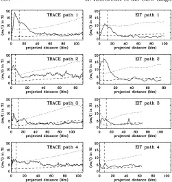
The fractional variabilityσa/I is plotted in Fig. 9 for the

Path 4

TRACE EIT

l vp(<20 Mm) vp (>20 Mm) vp αexp l vp (<20 Mm) vp(>20 Mm) vp αexp

(in km s−1_{) (in km s}−1₎

A 78±10 109±9 93±4 50◦−54◦ - - - -

-B 96±4 - 100±7 45◦−52◦ - - - -

-C 140±24 100±9 101±10 43◦−53◦ - - - -

-F 109±9 145±24 122±8 31◦−42◦ - - - -

-- - - A 110±11 165±34 124±12 45◦−54◦

D 66±3 97±36 86±3 54◦−57◦ - - - -

-- - - B 81±11 101±5 89±5 60◦−64◦

E 79±3 89±7 80±3 57◦−60◦ - - - -

-- - - C 80±11 105±7 96±12 56◦−64◦

- - - D 99±11 106±11 102±10 54◦−62◦

- - - E 144±17 131±14 138±14 38◦−50◦

- - - F 99±28 124±12 98±17 53◦−65◦

Fig. 8.The EUV intensity along path 4 as a function of time (horizontal axis) and distance along the path (vertical axis) in

the TRACE data (upper) and in the EIT data (lower) tracked in Fig. 2

times the fractional instrumental noise. As mentioned pre-viously,σaincludes various variability components. Hence

it cannot be interpreted as a measure of the change in am-plitude due to the PD only. For example, the peak present in the plots corresponding to path 3 (EIT) illustrates the contribution from a brightening to the variability. In the category of the brightenings we also find possible indica-tions of 5-min oscillaindica-tions (Fig. 6). Other contribuindica-tions to the variation of intensity are transverse loop oscillations. Their presence can be inferred from the difference images in Fig. 4. The places where field lines are sharply marked along the whole distance of the loop, indicate that the loops show a transverse motion.

3.4. Characteristics of a typical Propagating Disturbance (PD)

From different plots similar to Fig. 10, where the intensity during the whole sequence in a fixed point is plotted, we find the following characteristics of a PD:

1. The amplitude enhancements due to a passing distur-bance are typically 8% and 12% for the 195 ˚A, resp. 171 ˚A, wavelength of the background intensity. By measuring the intensity in that point just before (or af-ter) the PD passes we have an idea of the background intensity in a point;

Fig. 9.The fractional variability (σa/I) for the selected loops expressed in %I. The vertical line indicates the position of the footpoint. The dashed line corresponds to the instrumental noiseσn, the dotted line is three times the noise

time) of a disturbance. The typical duration of a PD passing a point in the TRACE data is 169 s. This is not to be confused with the decay-time, which expresses the total life-time of a PD while traveling along the loop;

3. We do not exclude the possibility that the disturbances are triggered by pulses or even by a periodical signal at the footpoints. However it is hard to decide, because the PDs are not always clear;

4. The PDs differ from brightenings since they are not stationary. They travel along the loops with a roughly constant speed. Speeds are measured in a time-space diagram (see Figs. 5 to 8) by measuring the slope of the diagonal ridges. Typical velocities are 110 km s−1

for EIT and 95 km s−1_{for TRACE. An acceleration of}

propagation is detected, in some cases, above the loop footpoint.

4. Discussion

We find outward propagating disturbances in virtually all loops within the opening bundle shown. Along some paths however we find more than one propagation speed, which we interpret as being due to the superposition of different loops.

In all cases studied, the PDs are weak disturbances, typically 8 and 12% of the background intensity resp. for the 195 ˚A and 171 ˚A, bandpass, which corresponds to a change of 2.8% resp. 3.5% of the background density. This means they are marginally detectable above the noise

Fig. 10.The temporal evolution near the footpoint of path 4.

The absolute intensity is plotted. The arrows point towards the intensities used to calculate the amplitude enhancement w.r.t. the background intensity due to a passing disturbance

level. This typical amplitude is convolved with the varying throughput bandpass efficiency as a function of temper-ature. Although detailed temperature diagnostics are be-yond the scope of the present paper, it seems most likely that these disturbances are formed closely to the peak for-mation temperature of the instruments bandpass. Suppose that a PD at a temperature significantly deviating from this peak formation temperature was detected, with an amplitude of the order of 10% of the background inten-sity. This would imply that another PD formed at the peak formation temperature, would have a significantly larger amplitude enhancement than 10% amplitude. None of this has been observed for many different PDs along many dif-ferent loops neither in the present data set nor by other authors (e.g. De Moortel et al. 2000). So, at least as a working hypothesis, is seems reasonable to assume that the PDs are formed at the peak formation temperature of the bandpass through which they are observed (1.6 MK for EIT (195 ˚A) and 1 MK for TRACE (171 ˚A)).

We can, in most cases, clearly distinguish a dominant direction of diagonal structure in all the time-space diagrams. This indicates that a dominant speed of prop-agation is present inside the loops. However, due to bad loop-tracking or perhaps the superposition of loops, we sometimes distinguish more than one velocity in an time-space diagram. Projected speeds found are typically 95 km s−1 _{for the 171 ˚A line and 110 km s}−1 _{for the}

195 ˚A line. The typical error on the measured speeds is 10 km s−1. The formal sound speed that correspond to these temperatures (192 km s−1 for EIT and 152 km s−1 for TRACE) are of the order of, but always higher than the observed propagation speeds. By interpreting the dif-ference between the derived sound speed and the observed propagation speed as exclusively due to a projection ef-fect, we can derive the necessary projection angle αexp.

These expected projection angles are consistent with the observed angles when the bundle of loops crossed the west-ern limb a few days later. This interpretation is possible sinceαexp lies in the acceptable range deduced by Fig. 3

(right) and because of the good correspondence between the angles measured in both wavelengths.

and EIT data set, we encounter here a conceptual prob-lem: how can the same wave give signatures at different temperatures traveling at different speeds? This hints at sharp temperature gradients in the selected paths: either the loops consist of concentric shells at different tempera-tures (e.g. Foukal 1976) or each “observed loop” consists of a bundle of very thin loop threads each at a differ-ent temperature (e.g. Aschwanden et al. 2000b; Fludra et al. 1997; Matthews & Harra-Murnion 1997). In both cases, the observations suggest that waves are triggered at the footpoints into the different shells or threads by the same source and propagate according to the sound speed of each shell or thread. Depending on the used bandpass this population of shells or threads is then convolved with the instrument bandpass, so that only those waves that travel along the loop at the peak formation temperature of the bandpass are seen. The observations show cases where the measured speeds of simultaneous PDs in both bandpasses are not consistent with the proposed explana-tion. This may be due to the superposition of loops where PDs from different depths in the field of view are com-pared, or due to less effective tracking of the loop due to transverse loop motions. Therefore, overlapping, multi-wavelength observations of longer duration and improved data-analysis techniques are desirable.

Although our present data set does not allow to ex-tend this reasoning much further, we are close here to

coronal seismology: trying to determine the internal coro-nal loop structure by studying the characteristics of the waves passing through it.

An alternative interpretation of the PDs as compared to the slow mode view is the hypothesis of plasma flows along the loop. Aschwanden et al. (2000) concluded from the properties of extensive loop systems as observed by TRACE, that they cannot be in static equilibrium, but in-stead harbour continual chromospheric upflows. The flow accelerates with height and may even become supersonic. The observation we have presented here show no system-atic acceleration of disturbances along the loop. The prop-agation speed of the PDs remain reasonably constant. Similar discussions on these two broad categories of inter-pretation (wave model vs. flow model) exist (e.g. Brekke et al. 1997).

As found in previous studies (e.g. Svestka et al. 1982a, 1982b) we find evidence of quasi-periodical triggering of the PDs at the footpoints. Reconnection caused by a flare as was found in e.g. Aschwanden et al. (1999) and Nakariakov et al. (1999) is also a valuable candidate as excitation mechanism. In a first inventory of this ac-tive region, based on the EIT data, there are only one strong brightening and several small brightenings detected around the footpoints of the loops here discussed (see Berghmans & Clette 1999).

We aim to compare the observations to analytical mod-els which model the propagation of sound waves in a coro-nal, isothermal loop structure, and study the feasibility of coronal diagnostics by such a method of comparison (Nakariakov et al. 2000).

Acknowledgements. The authors would like to thank the whole JOP80 team for their contribution to this unique data set. E. Verwichte, D. Berghmans and J. F. Hochedez would like to acknowledge the support of the Belgian Federal Services of Scientific, Technical and Cultural Affairs (SSTC/DWTC).

References

Aschwanden, M. J., Fletcher, L., Schrijver, C. J., & Alexander, D. 1999, ApJ, 520, 880

Aschwanden, M. J., Nightingale, R. W., Tarbell, T. D., & Wolfson, C. J. 2000, ApJ, 535, 1027

Aschwanden, M. J., Nightingale, R. W., & Alexander, D. 2000, ApJ, 541, 1059

Berghmans, D., Clette, F., & Moses, D. 1998, A&A, 336, 1039 Berghmans, D., & Clette, F. 1999, Sol. Phys., 186, 207 Brekke, P., Kjeldseth-Moe, O., & Harrison, R. A. 1997, Sol.

Phys., 175, 511 Clette, F., et al. 1998,

http://sohowww.nascom.nasa.gov/soc/JOPs/jop080.txt

Delaboudini`ere, J.-P., et al. 1995, Sol. Phys., 162, 291 De Moortel, I., Ireland, J., & Walsh, R. W. 2000, A&A, 355,

L23

DeForest, C. E., & Gurman, J. B. 1998, ApJ, 501, L217 Fludra, A., et al. 1997, Sol. Phys., 175, 487

Foukal, P. V. 1976, ApJ, 210, 575

Handy, B. N., et al. 1999, Sol. Phys., 187, 229 Harrison, R. A. 1987, A&A, 182, 337

Harrison, R. A. 1997, in Proc of the 5th SoHO Workshop, Oslo, June 1997, ESA SP-404, 7

Harrison, R. A. 1997, Sol. Phys., 175, 467

Innes, D. E., Inhester, B., Axford, W. I., & Whilhelm, K. 1997, Nature, 386(24), 811

Kjeldseth-Moe, & Brekke, P. 1998, Sol. Phys., 182, 73 Martin, S. F., & Svestka, Z. F. 1988, Sol. Phys., 116, 91 Matthews, S. A., & Harra-Murnion, L. K. 1997, Sol. Phys.,

175, 541

Nakariakov, V. M., Ofman, L., Deluca, E., Roberts, B., & Davila, J. M. 1999, Science, 285, 862

Nakariakov, V. M., Verwichte, E., Berghmans, D., & Robbrecht, E. 2000, A&A, 362, 1151

Nightingale, R. W., Aschwanden, M. J., & Hurlburt, N. E. 1999, Sol. Phys., 190, 249

Ofman, L., Nakariakov, V. M., & DeForest, C. E. 1999, ApJ, 514, 441

Ofman, L., Nakariakov, V. M., & Sehgal, N. 2000, ApJ, 533, 1071

Priest, E. 1984, Solar Magnetohydrodynamics (D. Reidel Publ. Co., Dordrecht, Holland)

Reale, F., Peres, G., & Serio, S. 2000, ApJ, 535, 412

Robbrecht, E., Berghmans, D., & Poedts, S. 1999, Proc. of the 8th SOHO Workshop, Paris, June 1999, ESA SP-446, 575 Roberts, B., Edwin, P. M., & Benz, A. O. 1984, ApJ, 279, 857 Shimojo, M., Shibata, K., Hori, K., & Yokoyama, T. 1998, Proc. of an international conference meeting in Guadeloupe, France, ESA SP-421, 163

Svestka, Z., et al., and 8 co-authors, 1982, Sol. Phys., 75, 305 Svestka, Z., et al. 1982, Sol. Phys., 80, 143

Svestka, Z., Farnik, F., Fontenla, J. M., & Martin, S. F. 1989, Sol. Phys., 123, 317

Svestka, Z. 1994, Sol. Phys., 152, L505