Experiments in Sentence Language Identification with Groups of Similar
Languages
Ben King Department of EECS University of Michigan
Ann Arbor
Dragomir Radev Department of EECS School of Information University of Michigan
Ann Arbor
Steven Abney Department of Linguistics
University of Michigan Ann Arbor
Abstract
Language identification is a simple problem that becomes much more difficult when its usual assumptions are broken. In this paper we consider the task of classifying short segments of text in closely-related languages for the Discriminating Similar Languages shared task, which is broken into six subtasks, (A) Bosnian, Croatian, and Serbian, (B) Indonesian and Malay, (C) Czech and Slovak, (D) Brazilian and European Portuguese, (E) Argentinian and Peninsular Spanish, and (F) American and British English. We consider a number of different methods to boost classification performance, such as feature selection and data filtering, but we ultimately find that a simple na¨ıve Bayes classifier using character and wordn-gram features is a strong baseline that is difficult to improve on, achieving an average accuracy of 0.8746 across the six tasks.
1 Introduction
Language identification constitutes the first stage of many NLP pipelines. Before applying tools trained on specific languages, one must determine the language of the text. It is also is often considered to be a solved task because of the high accuracy of language identification methods in the canonical formulation of the problem with long monolingual documents and a set of mostly dissimilar languages to choose from. We consider a different setting with much shorter text in the form of single sentences drawn from very similar languages or dialects.
This paper describes experiments related to and our submissions to the Discriminating Similar Lan-guages (DSL) shared task. This shared task has six subtasks, each a classification task in which a sentence must be labeled as belonging to a small set of related languages:
• Task A: Bosnianvs.Croatianvs.Serbian
• Task B: Indonesianvs.Malay
• Task C: Czechvs.Slovak
• Task D: Brazilianvs.European Portuguese
• Task E: Argentinianvs.Peninsular Spanish
• Task F: Americanvs.British English
The first three tasks involve classes that could be rightly called separate languages or dialects. The classes of each of the final three tasks have high mutual intelligibility and are so similar that some linguists may not even classify them as separate dialects. We will use the term “language variant” to refer to such classes.
In this paper we experiment with several types of methods aimed at improving the classification ac-curacy of these tasks: machine learning methods, data pre-processing, feature selection, and additional training data. We find that a simple na¨ıve Bayes classifier using character and wordn-gram features is a strong baseline that is difficult to improve on. Because this paper covers so many different types of methods, its format eschews the standard “Results” section, instead providing comparisons of methods as they are presented.
This work is licenced under a Creative Commons Attribution 4.0 International License. Page numbers and proceedings footer are added by the organizers. License details:http://creativecommons.org/licenses/by/4.0/
2 Related Work
Recent directions in language identification have included finer-grained language identification (King and Abney, 2013; Nguyen and Dogruoz, 2013; Lui et al., 2014), language identification for microblogs (Bergsma et al., 2012; Carter et al., 2013), and the task of this paper, language identification for closely related languages.
Language identification for closely related languages has been considered by several researchers, though it has lacked a systematic evaluation before the DSL shared task. The problem of distinguish-ing Croatian from Serbian and Slovenian is explored by Ljubeˇsi´c et al. (2007), who used a list of most frequent words along with a Markov model and a word blacklist, a list of words that are not allowed to appear in a certain language. A similar approach was later used by Tiedemann and Ljubeˇsi´c (2012) to distinguish Bosnian, Croatian, and Serbian. They further develop the idea of a blacklist classifier, loosening the binary restriction of the earlier work’s blacklist and considering the frequencies of words rather than their absolute counts. This blacklist classifier is able to outperform a na¨ıve Bayes classifier with large amounts of training data. They also find training on parallel data to be important, as it al-lows the machine learning methods to pick out features relating to the differences between the languages themselves, rather than learning differences in domain.
Zampieri et al. consider classes that would be most often classified as language varieties rather than separate languages or dialects (Zampieri et al., 2012; Zampieri and Gebrekidan, 2012; Zampieri et al., 2013). A similar problem of distinguishing among Chinese text from mainland China, Singapore, and Taiwan is considered by Huang and Lee (2008) who approach the problem by computing similarity between a document and a corpus according to the size of the intersection between the sets of types in each.
A similar, but somewhat different problem of automatically identifying lexical variants between closely related languages is considered in (Peirsman et al., 2010). Using distributional methods, they are able to identify Netherlandic Dutch synonyms for words from Belgian Dutch.
3 Data
This paper’s training data and evaluation data both come from the DSL corpus collection (DSLCC) (Tan et al., 2014). We use the training section of this data for training and the development section for evaluation. The training section consists of 18,000 labeled instances per class, while the development section has 2,000 labeled instances per class.
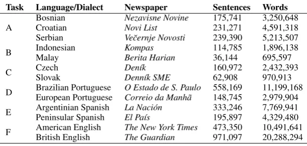
In order to try to increase classifier accuracy (and to avoid the problems with the task F training data), we decided to collect additional training data for each open-class task. For each task, we collected newspaper text from the appropriate websites for each of the 2–3 languages. We used regular expressions to split the text into sentences, and created a set of rules to filter out strings that were unlikely to be good sentences. Because the pages on the newspaper websites tended to have some boilerplate text, we collated all the sentences and only kept one copy of each sentence.
Task Language/Dialect Newspaper Sentences Words
[image:2.595.145.451.596.742.2]A BosnianCroatian Nezavisne NovineNovi List 175,741231,271 3,250,6484,591,318 Serbian Ve˘cernje Novosti 239,390 5,213,507 B IndonesianMalay KompasBerita Harian 114,78536,144 1,896,138695,597 C CzechSlovak Den´ıkDenn´ık SME 160,97262,908 2,432,393970,913 D Brazilian PortugueseEuropean Portuguese O Estado de S. PauloCorreio da Manh˜a 558,169148,745 11,199,1682,979,904 E Argentinian SpanishPeninsular Spanish La Naci´onEl Pa´ıs 333,246195,897 7,769,9414,329,480 F American EnglishBritish English The New York TimesThe Guardian 473,350971,097 10,491,64120,288,294
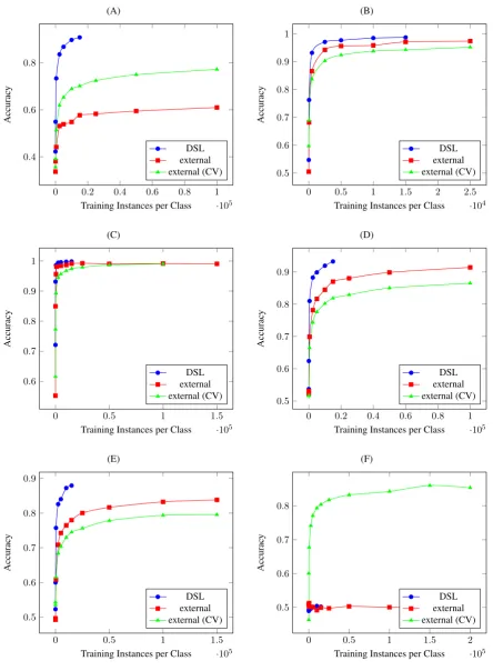
In order to create balanced training data, for each task we downsampled the number of sentences of the larger collection(s) to match the number of sentences in the smaller collection. For example, we downsampled the British English collection to 473,350 sentences and combined it with the American English sentences to create the training data for English. Figure 1 shows results of training using this external data.
3.1 Features
We use many types of features that have been found to be useful in previous language identification work: word unigrams, word bigrams, and charactern-grams (2≤n≤6). Charactern-grams are simply substrings of the sentence and may include in addition to letters, whitespace, punctuation, digits, and anything else that might be in the sentence. Words, for the purpose of word unigrams and bigrams, are simply maximal tokens not containing any punctuation, digit, or whitespace.
When instances are encoded into feature vectors, each feature has a value equal to the number of times it occured in the corresponding sentence, so the majority of features have a value of 0 for any given instance, but it is possible for a feature to occur multiple times in a sentence and have a value greater than 1.0 in the feature vector. Table 2 below compares the performance of a na¨ıve Bayes classifier using each of the different feature groups below.
Word Character
Task All 1 2 2 3 4 5 6
Bosnian/Croatian/Serbian 0.9348 0.9290 0.8183 0.7720 0.8808 0.9412 0.9338 0.9323 Indonesian/Malay 0.9918 0.9943 0.9885 0.8545 0.9518 0.9833 0.9908 0.9930 Czech/Slovak 0.9998 1.0000 0.9985 0.9980 0.9998 0.9998 1.0000 1.0000 Portuguese 0.9535 0.9468 0.9493 0.7935 0.8888 0.9318 0.9468 0.9570 Spanish 0.8623 0.8738 0.8625 0.7673 0.8273 0.8513 0.8610 0.8660 English 0.4970 0.4948 0.5005 0.4825 0.4988 0.5010 0.5048 0.4993 Average 0.8732 0.8731 0.8529 0.7780 0.8412 0.8681 0.8729 0.8746
Table 2: Accuracies compared for different sets of features compared. The classifier used here is na¨ıve Bayes.
4 Methods
Our baseline method against which we compare all other models is a na¨ıve Bayes classifier using word unigram features trained on the DSL-provided training data. The methods we compare to it can be broken into three classes: other machine learning methods, feature selection methods, and data filtering methods.
The classification pipeline used here has the following stages: (1) data filtering, (2) feature extraction, (3) feature selection, (4) training, and (5) classification.
4.1 Machine Learning Methods
We will use the following notation throughout this section. An instance x, that is, a sentence to be classified, with a corresponding class label y is encoded into a feature vector f(x), where each entry is an integer denoting how many times the feature corresponding to that entry’s index occurred in the sentence. The class label here is a language and it’s drawn from a small sety∈ Y.
In addition to the na¨ıve Bayes classifier, we also experiment with two versions of logistic regression and a support vector machine classifier. The MALLET machine learning library implementations are used for the first three classifiers (McCallum, 2002) and SVMLight is used for the fourth (Joachims, ).
P(y|f(x)) = P(f1(x))P(y)Yn i=1
P(f(x)i|y) (1)
As na¨ıve Bayes is a generative classifier, it has been shown to be able to outperform discriminative classifiers when the number of training instances is small compared to the number of features (Ng and Jordan, 2002). This classifier is additionally advantageous in that it has a simple closed-form solution for maximizing its log likelihood.
Logistic Regression A logistic regression classifier is a discriminative classifier whose parameters are encoded in a vectorθ. The conditional probability of a class label over an instance(x, y)is modeled as follows:
P(y|x;θ) = Z(x1;θ)exp{f(x, y)·θ} ; Z(x, θ) = X y∈Y
exp{f(x, y)·θ} (2)
The parameter vectorθis commonly estimated by maximizing the log-likelihood of this function over the set of training instances(x, y)∈ T in the following way:
θ= argmaxθ X
(x,y)∈T
logP(yi|xi;θ)−λR(θ) (3)
The term R(θ) above is a regularization term. It is common for such a classifier to overfit the pa-rameters to the training data. To keep this from happening, a regularization term can be added which keeps the parameters inθfrom growing too large. Two common choices for this function are L2 and L1 normalization:
RL2 =||θ||22 =
n X
i=1 θ2
i , RL1 =||θ||1 =
n X
i=1
|θi| (4)
L2 regularization is well-grounded theoretically, as it is equivalent to a model with a Gaussian prior on the parameters (Rennie, 2004). But L1 regularization has a reputation for enforcing sparsity on the parameters. In fact, it has been shown to be quite effective when the number of irrelevant dimensions is greater than the number of training examples, which we expect to be the case with many of the tasks in this paper (Ng, 2004).
Support Vector Machines A support vector machine (SVM) is a type of linear classifier that attempts to find a boundary that linearly separates the training data with the maximum possible margin. SVMs have been shown to be a very efficient and high accuracy method to classify data across a wide variety of different types of tasks (Tsochantaridis et al., 2004).
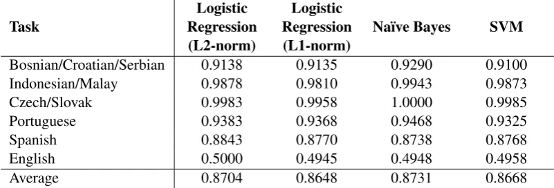
Table 3 below compares these machine learning methods. Because of its consistently good perfor-mance across tasks, we use a na¨ıve Bayes classifier throughout the rest of the paper.
4.2 Feature Selection Methods
We expect that the majority of features are not relevant to the classification task, and so we experimented with several methods of feature selection, both manual and automatic.
Information Gain As a fully automatic method of feature extraction, we used information gain to score features according to their expected usefulness. Information gain (IG) is an information theoretic concept that (colloquially) measures the amount of knowledge about the class label that is gained by having access to a specific feature. Iff is the occurence an individual feature andf¯the non-occurence of a feature, we measure its information gain by the following formula:
G(f) =P(f)
X
y∈Y
P(y|f)logP(y|f)
+P( ¯f)
X
y∈Y
logP(y|f¯)logP(y|f¯)
Task RegressionLogistic (L2-norm)
Logistic Regression
(L1-norm) Na¨ıve Bayes SVM
Bosnian/Croatian/Serbian 0.9138 0.9135 0.9290 0.9100
Indonesian/Malay 0.9878 0.9810 0.9943 0.9873
Czech/Slovak 0.9983 0.9958 1.0000 0.9985
Portuguese 0.9383 0.9368 0.9468 0.9325
Spanish 0.8843 0.8770 0.8738 0.8768
English 0.5000 0.4945 0.4948 0.4958
[image:5.595.98.499.63.199.2]Average 0.8704 0.8648 0.8731 0.8668
Table 3: Comparison of different machine learning methods using word unigram features on the six tasks.
To reduce the number of features being used in classification (and to hopefully remove irrelevant features), we choose the 10,000 features with the highest IG scores. IG considers each feature indepen-dently, so it is possible that redundant feature sets could be chosen. For example, it might happen that both the quadrigramtherand the trigramthescore highly according to IG and are both selected, even though they are highly correlated with one another.
Parallel Text Feature Selection Because IG feature selection often seemed to choose features more related to differences in domain than to differences in language (see Table 7), we wanted to try to isolate features that are specific to language differences. It has been shown in previous work that training on parallel text can help to isolate language differences since the domains of the languages are identical (Tiedemann and Ljubeˇsi´c, 2012). For each of the tasks,1 we use translations of the complete Bible as a
parallel corpus, running IG feature selection exactly as above. Table 4 below gives more details about the texts used.
Task Language/Dialect Bible
B IndonesianMalay Alkitab dalam Bahasa Indonesia Masa Kini2001 Today’s Malay Version C CzechSlovak Cesk´y studijn´ı prekladSlovensk´y Ekumenick´y Biblia
D Brazilian PortugueseEuropean Portuguese a B´IBLIA para todosAlmeida Revista e Corrigida (Portugal) E Argentinian SpanishPeninsular Spanish La Palabra (versi´on hispanoamericana)La Palabra (versi´on espa˜nola) F American EnglishBritish English New International VersionNew International Version Anglicized
Table 4: Bibles used as parallel corpora for feature selection.
Manual Feature Selection We also used manual feature selection, selecting features to use in the clas-sifiers from lists published on Wikipedia comparing the two languages. Of course some of the features in lists like these are features that are quite difficult to detect using NLP (especially before the language has been identified) such as characteristic passive or genitive constructions. But there are many features that we are able to detect and use in a list of manually selected features, such as charactern-grams relating to morphology and spelling and wordn-grams relating to vocabulary differences.
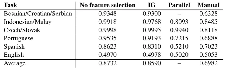
Table 5 below compares these feature selection methods on each task. Since the manual feature selec-tion suggested all types of features, including charactern-gram and word unigram and bigram features, the experiments in this section use all features described in Section 3.1. The results show that any type of feature selection consistently hurts performance, though IG hurts the least, and it should be noted that in certain cases with other machine learning methods, IG feature selection actually yielded better
performance than all features. That the feature selection methods designed to isolate language-specific features performed so poorly is one indicator that the labeled data has additional differences that are not tied to the languages themselves. We discuss this idea further in Section 5.
Task No feature selection IG Parallel Manual
Bosnian/Croatian/Serbian 0.9348 0.9300 – 0.6328 Indonesian/Malay 0.9918 0.9768 0.8093 0.8485
Czech/Slovak 0.9998 0.9995 0.9940 0.8118
Portuguese 0.9535 0.9193 0.7215 0.6888
Spanish 0.8623 0.8310 0.5210 0.7023
English 0.4970 0.4978 0.5020 0.5053
Average 0.8732 0.8590 – 0.6982
Table 5: Comparison of manual and automatic feature selection methods. IG and parallel feature selec-tion both use the 10,000 features with the highest IG scores.
4.3 Data Filtering Methods
English Word Removal In looking through the training data for the non-English tasks, we observed that it was not uncommon for sentences in these languages to contain English words and phrases. Be-cause foreign words should be independent of the language/dialect used, English words included in the sentences for other tasks should just be noise that, if removed will improve classification performance.
For each of the non-English tasks (A, B, C, D, and E), we create a new training set for identifying English/non-English words by mixing together 1,000 random English words with 10,000 random task-language words. The imbalance in the classes is a compromise, approximating the actual proportions in the test without leading to a degenerate classifier. Because English and the other classes are so dissimilar, the performance of the English word classifier is very insensitive to the actual ratio. From this data, we train a na¨ıve Bayes classifier using character 3-grams, 4-grams, and 5-grams.
We manually labeled the words of 150 sentences from the five non-English tasks in order to evaluate the English word classifier. Across the five tasks, the precision was 0.76 and the recall was 0.66, leading to an F1-score of 0.70. Any words labeled as English by the classifier were removed from the sentence and it was passed on to the feature extraction, classification, and training stages.
Named Entity Removal We also observed another common class of word that could potentially act as a noise source: named entities. Across all the languages listed studied here, it is common for named entities to begin with a capital letter. Lacking named entity recognizers for all the languages here, we instead used the property of having an initial capital letter as a surrogate for recognizing a word as a named entity. Because all the languaes studied here also have the convention of capitalizing the first word of a sentence, we remove all words beginning with a capital letter except for the first and pass this abridged sentence on to the feature extraction, classification, and training stages.
Task No data filtering English WordRemoval Named EntityRemoval
Bosnian/Croatian/Serbian 0.9138 0.9105 0.9003
Indonesian/Malay 0.9878 0.9885 0.9778
Czech/Slovak 0.9983 0.9980 0.9973
Portuguese 0.9383 0.9365 0.9068
Spanish 0.8843 0.8835 0.8555
English 0.5000 0.5000 0.5050
[image:6.595.115.487.113.225.2]Average 0.8704 0.8695 0.8571
(A)
0 0.2 0.4 0.6 0.8 1 ·105
0.4 0.6 0.8
Training Instances per Class
Accurac y DSL external external (CV) (B)
0 0.5 1 1.5 2 2.5 ·104
0.5 0.6 0.7 0.8 0.9 1
Training Instances per Class
Accurac y DSL external external (CV) (C)
0 0.5 1 1.5
·105
0.6 0.7 0.8 0.9 1
Training Instances per Class
Accurac y DSL external external (CV) (D)
0 0.2 0.4 0.6 0.8 1 ·105
0.5 0.6 0.7 0.8 0.9
Training Instances per Class
Accurac y DSL external external (CV) (E)
0 0.5 1 1.5
·105
0.5 0.6 0.7 0.8 0.9
Training Instances per Class
Accurac y DSL external external (CV) (F)
0 0.5 1 1.5 2
·105
0.5 0.6 0.7 0.8
Training Instances per Class
Accurac
y
[image:7.595.82.527.66.671.2]DSL external external (CV)
Bosnian/Croatian/Serbian Indonesian/Malay Czech/Slovak Portuguese Spanish English
da bisa sa Portugal the I
kako berkata se R Rosario you
sa kerana aj euros han The
kazao karena ako Brasil euros said
takode daripada ve cento Argentina Obama
rekao saat pre governo PP your
evra dari pro Lusa Fe If
tijekom beliau ktor´e PSD Rajoy that
posle selepas s´u Ele Espa˜na but
posto bahwa ktor´y Governo Madrid It
Table 7: The ten word-unigram features given the highest weight by information gain feature selection for each of the six tasks.
5 Discussion
Across many of the tasks, there was evidence that performance was tied more strongly to domain-specific features of the two classes rather than to language- (or language-variant-) specific features. For example, Table 7 shows the best word-unigram features selected by information gain feature selection for each of the tasks. The Portuguese, Spanish, and English tasks specifically have as many of their most important features named entities and other non-language specific features.
It seems that for many of the tasks, it is easier to distinguish the subject matter written about than it is to distinguish the languages/dialects themselves. With Portuguese, for example, Brazilian dialect speakers were much more likely to discuss places in Brazil and mention Brazilian reais (currency, abbreviated as R), while European speakers mentioned euros, places in Portugal, and discussed Portuguese politics. While there are definite linguistic differences between Brazilian and European Portuguese, these seem to be less pronounced than the superficial differences in subject matter.
Practically, this is not necessarily a bad thing for this shared task, as the domain information gives extra clues that allow the task to be completed with higher accuracy than would otherwise be possible. This would become problematic if one wanted to apply a classifier trained on this data to general domains, where the classifier may not be able to rely on the speaker talking about a certain subject matter. To address this, the classifier would either need to focus on features specific to the language pair itself or would need to be trained on data that spanned many domains.
Further evidence of domain overfitting comes from the fact that the larger training sets drawn from newspaper text were not able to improve performance on the development set over the provided training data, which is presumably drawn from the same collection as the development data. Figure 1 shows learning curves for each of the six tasks. Though all the external text is self-consistent (cross-validation results in high accuracy), in none of the cases does training on a large amount of external data allow the classifier to exceed the accuracy achieved by training on the DSL data.
6 Conclusion
References
Shane Bergsma, Paul McNamee, Mossaab Bagdouri, Clayton Fink, and Theresa Wilson. 2012. Language identi-fication for creating language-specific twitter collections. InProceedings of the Second Workshop on Language in Social Media, pages 65–74. Association for Computational Linguistics.
Simon Carter, Wouter Weerkamp, and Manos Tsagkias. 2013. Microblog language identification: Overcoming the limitations of short, unedited and idiomatic text. Language Resources and Evaluation, 47(1):195–215. Chu-Ren Huang and Lung-Hao Lee. 2008. Contrastive approach towards text source classification based on
top-bag-of-word similarity. pages 404–410.
Thorsten Joachims. Svmlight: Support vector machine. http://svmlight. joachims. org/.
Ben King and Steven Abney. 2013. Labeling the languages of words in mixed-language documents using weakly supervised methods. InProceedings of NAACL-HLT, pages 1110–1119.
Nikola Ljubeˇsi´c, Nives Mikeli´c, and Damir Boras. 2007. Language identication: How to distinguish similar languages? InProceedings of the 29th International Conference on Information Technology Interfaces, pages 541–546.
Marco Lui, Jey Han Lau, and Timothy Baldwin. 2014. Automatic detection and language identification of multi-lingual documents.Transactions of the Association for Computational Linguistics, 2:27–40.
Andrew K. McCallum. 2002. Mallet: A machine learning for language toolkit.
http://mallet.cs.umass.edu.
Andrew Y Ng and Michael I Jordan. 2002. On discriminative vs. generative classifiers: A comparison of logistic regression and naive bayes.Advances in neural information processing systems, 2:841–848.
Andrew Y Ng. 2004. Feature selection, l 1 vs. l 2 regularization, and rotational invariance. InProceedings of the twenty-first international conference on Machine learning, page 78. ACM.
Dong-Phuong Nguyen and A Seza Dogruoz. 2013. Word level language identification in online multilingual communication. Association for Computational Linguistics.
Yves Peirsman, Dirk Geeraerts, and Dirk Speelman. 2010. The automatic identification of lexical variation between language varieties. Natural Language Engineering, 16(4):469–491.
Jason Rennie. 2004. On l2-norm regularization and the gaussian prior.
http://people.csail.mit.edu/jrennie/writing.
Liling Tan, Marcos Zampieri, Nikola Ljubeˇsic, and J¨org Tiedemann. 2014. Merging comparable data sources for the discrimination of similar languages: The dsl corpus collection. InProceedings of The 7th Workshop on
Building and Using Comparable Corpora (BUCC).
J¨org Tiedemann and Nikola Ljubeˇsi´c. 2012. Efficient discrimination between closely related languages. In
COLING, pages 2619–2634.
Ioannis Tsochantaridis, Thomas Hofmann, Thorsten Joachims, and Yasemin Altun. 2004. Support vector ma-chine learning for interdependent and structured output spaces. InProceedings of the twenty-first international
conference on Machine learning, page 104. ACM.
Marcos Zampieri and Binyam Gebrekidan. 2012. Automatic identification of language varieties: The case of portuguese. InProceedings of KONVENS, pages 233–237.
Marcos Zampieri, Binyam Gebrekidan Gebre, and Sascha Diwersy. 2012. Classifying pluricentric languages: Extending the monolingual model. In Proceedings of the Fourth Swedish Language Technlogy Conference
(SLTC2012), pages 79–80.