Bankruptcy Prediction Using Machine Learning

ISSN Online: 2162-2442 ISSN Print: 2162-2434

DOI: 10.4236/jmf.2017.74049 Nov. 17, 2017 908 Journal of Mathematical Finance

Bankruptcy Prediction Using Machine Learning

Nanxi Wang

Shanghai Starriver Bilingual School, Shanghai, China

Abstract

With improved machine learning models, studies on bankruptcy prediction show improved accuracy. This paper proposes three relatively newly-developed methods for predicting bankruptcy based on real-life data. The result shows among the methods (support vector machine, neural network with dropout, autoencoder), neural network with added layers with dropout has the highest accuracy. And a comparison with the former methods (logistic regression, genetic algorithm, inductive learning) shows higher accuracy.

Keywords

Support Vector Machine, Autoencoder, Neural Network, Bankruptcy, Machine Learning

1. Introduction

Machine learning is a subfield of computer science. It allows computers to build analytical models of data and find hidden insights automatically, without being unequivocally coded. It has been applied to a variety of aspects in modern socie-ty, ranging from DNA sequences classification, credit card fraud detection, robot locomotion, to natural language processing. It can be used to solve many types of tasks such as classification. Bankruptcy prediction is a typical example of clas-sification problems.

Machine learning was born from pattern recognition. Earlier works of the same topic (machine learning in bankruptcy) use models including logistic re-gression, genetic algorithm, and inductive learning.

Logistic regression is a statistical method allowing researchers to build predic-tive function based on a sample. This model is best used for understanding how several independent variables influence a single outcome variable [1]. Though useful in some ways, logistic regression is also limited.

Genetic algorithm is based on natural selection and evolution. It can be used

How to cite this paper: Wang, N.X. (2017) Bankruptcy Prediction Using Machine Learning. Journal of Mathematical Finance, 7, 908-918.

https://doi.org/10.4236/jmf.2017.74049

Received: August 30, 2017 Accepted: November 14, 2017 Published: November 17, 2017

Copyright © 2017 by author and Scientific Research Publishing Inc. This work is licensed under the Creative Commons Attribution International License (CC BY 4.0).

DOI: 10.4236/jmf.2017.74049 909 Journal of Mathematical Finance to extract rules in propositional and first-order logic, and to choose the appro-priate sets of if-then rules for complicated classification problems [2].

Inductive learning’s main category is decision tree algorithm. It identifies training data or earlier knowledge patterns and then extracts generalized rules which are then used in problem solving [2].

To see if the accuracy of bankruptcy prediction can be further improved, we propose three latest models—support vector machine (SVM), neural network, and autoencoder.

Support vector machine is a supervised learning method which is especially effective in cases of high dimensions, and is memory efficient because it uses a subset of training points in the decision function. Also, it specifies kernel func-tions according to the decision function [3]. Its nice math property guarantees a simple convex optimization problem to converge to a single global problem.

Neural networks, unlike conventional computers, are expressive models that learn by examples. They contain multiple hidden layers, thus are capable of learning very complicated relationships between inputs and outputs. And they operate significantly faster than conventional techniques. However, due to li-mited training data, overfitting will affect the ultimate accuracy. To prevent this, a technique called dropout—temporarily and randomly removes units (hidden and visible)—to the neural network [4].

Autoencoder, also known as Diabolo network, is an unsupervised learning al-gorithm that sets the target values to be equal to the inputs. By doing this, it suppresses the computation of representing a few functions, which improves accuracy. Also, the amount of training data required to learn these functions is reduced [5].

This paper is structured as follows. Section 2 describes the motivation for this idea. Section 3 describes relevant previous work. Section 4 formally describes the three models. In Section 5 we present our experimental results where we do a parallel comparison within the three models we choose and a longitudinal com-parison with the three older models. Section 6 is the conclusion. Section 7 is the reference.

2. Motivation

The three models we choose (SVM, neural network, autoencoder) are relatively newly-developed but have already been applied to many fields.

SVM has been used successfully in many real-world problems such as text ca-tegorization, object tracking, and bioinformatics (Protein classification, Cancer classification). Text categorization is especially helpful in daily life—web searching and email filtering provide huge convenience and work efficiency.

DOI: 10.4236/jmf.2017.74049 910 Journal of Mathematical Finance Autoencoders are especially successful in solving difficult tasks like natural language processing (NLP). They have been used to solve the previous seemingly intractable problems in NLP, including word embeddings, machine translation, document clustering, sentiment analysis, and paraphrase detection.

However, the usage of the three models in economics or finance is compara-tively hard to find. So, we aim to find out if they still work well in economical field by running them with real-life data in a predicting bankruptcy task.

Another motivation is finding out if the accuracy of this particular problem (bankruptcy prediction) can be improved after reading previous works—The discovery of experts’ decision rules from qualitative bankruptcy data using ge-netic algorithms [2], and Predicting Bankruptcy with Robust Logistic Regression [1]—which uses older models. Thus, a comparison of the models and results is included in this paper.

3. Related Work

Machine learning enables computers to find insights from data automatically. The idea of using machine learning to predict bankruptcy has previously been used in the context of Predicting Bankruptcy with Robust Logistic Regression by Richard P. Hauser and David Booth [1]. This paper uses robust logistic regres-sion which finds the maximum trimmed correlation between the samples re-mained after removing the overly large samples and the estimated model using logistic regression [1]. This model has its limitation. The value of this technique relies heavily on researchers’ abilities to include the correct independent va-riables. In other words, if researchers fail to identify all the relevant independent variables, logistic regression will have little predictive value [7]. Its overall accu-racy is 75.69% in the training set and 69.44% in testing set.

Another work, the discovery of experts’ decision rules from qualitative bank-ruptcy data using genetic algorithms, in 2003 by Myoung-Jong Kim and Ingoo Han uses the same dataset as we do. They apply older models—inductive learn-ing algorithms (decision tree), genetic algorithms, and neural networks without dropout. Since the length of genomes in GA is fixed, a given problem cannot easily be encoded. And GA gives no guarantee of finding the global maxima. The problem of inductive learning is with the one-step-ahead node splitting without backtracking, which may generate a suboptimal tree. Also, decision trees can be unstable because small variations in the data might result in a completely differ-ent tree being generated [3]. And the absence of dropout in the neural network model increases the possibility of overfitting which affects accuracy. The overall accuracies are 89.7%, 94.0%, and 90.3% respectively.

The models we choose either contain a newly developed technique, like dro-pout, or completely new models that have hardly been utilized in bankruptcy prediction.

4. Model Description

DOI: 10.4236/jmf.2017.74049 911 Journal of Mathematical Finance

4.1. Support Vector Machine

Specifically, we use support vector classify (SVC), a subcategory of SVM, in this task. It constructs a hyper-plane, as shown in Figure 1, in a high dimensional space which is used for classification. Generally, a good separation represented by the solid line in Figure 1 means the distance(the space between the dotted lines) to the nearest training data points (the red and blue dots) of any class (represented by the color red and blue) is the largest. This is also known as func-tional margin [3].

With training vectors in two classes and a vector,

{

}

, 1, , , 1, 1n p

i

x ∈ i=  n y∈ −

respectively, SVM aims at solving the problem:

T , ,

1

1 min

2

n

i b

i

C

ω ζ ω ω+

∑

subject to

( )

(

)

1

i i i

y ω φ x +b ≥ −ζ

Its dual is

T T

1 min

2 Q e

α α α− α

subject to

T

0, 0 _i , 1, ,

y α= ≤α ≤C i=  n

where e is a common vector, C>0 is upper bound, Q is n by n positive semi-definite matrix, Qij ≡y y k x xi j

(

)

(

)

( )

( )

T

,

i j i j

K x x =φ x φ x is the kernel.

DOI: 10.4236/jmf.2017.74049 912 Journal of Mathematical Finance Here the function implicitly maps the training vectors into a higher dimensional space.

The decision function is:

(

)

1

sgn , n

i i i

i

yαK x x ρ

=

 ₊ 

 



∑

4.2. Neural Network with Dropout

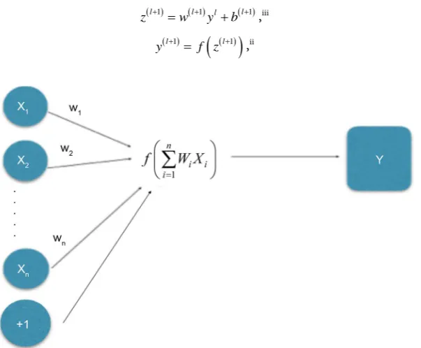
Neural networks’ inputs are modelled as layers of neurons. Its structure is shown in the following figure.

As shown in Figure 1, the formal neuron uses n inputs x x1, 2,,xn to clas-sify the signals coming from dendrites, and are then synoptically weighted cor-respondingly with w w1, 2,,wn that measure their permeabilities. Then, the excitation level of the neuron is calculated as the weighted sum of input values:

1

n

i i i

w x ξ

=

=

∑

f in Figure 2 represents activation function.

When the value of excitation level x reaches the threshold h, the output y (state) of the neuron is induced. This simulates the electric impulse generated by axon [8].

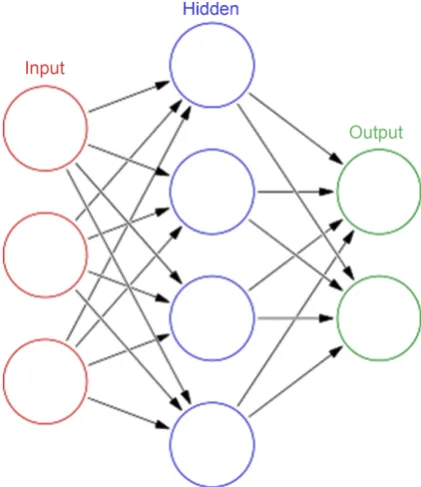
Dropout is a technique that further improves neural network’s accuracy. In Figure 3, let L be the number of hidden layers, l∈

{

}

the neural network, z l

( )

( )

l, respectively. W l

( )

( )

{

}

l∈  L− and any hidden unit i, the network then can be described as:

( )l1 ( )l1 l ( )l1

z + =w + y +b + ,iii

( )l1

( )

y + = f z + ,ii

DOI: 10.4236/jmf.2017.74049 913 Journal of Mathematical Finance

Figure 3. Artificial neural network.

where f is any activation function.

With dropout, the feed-forward operation becomes: r(l)_{-Bernoulli(p), j}

( )l ( ) ( )l l

y =r y ,

( )l1 ( )l1 l ( )l1 z + =w + y +b + ,iii[4].

4.3. Autoencoder

Consider an n/p/n autoencoder.

In Figure 4, let F and G denote sets, n and p be positive integers where 0 < p < n, and B be a class of functions from Fn _{to G}p_.

Define X =

{

}

{

}

over Fn_.

For any A∈_{A and B}∈_{B, the input vector x}∈_Fn _{becomes output vector A◦}

B(x) ∈_Fn _{through the autoencoder. The goal is to find A ∈A and B∈B that}

minimize the overall distortion function:

(

)

( )

( )

min ,E A B =minE x_t =min∆A B x _t ,x_t [10].

4.4. Decision Tree

Given training vectors n i

x∈R , i=1,,l and a label vector y∈Rl, a decision

tree groups the sample according to the same labels.

DOI: 10.4236/jmf.2017.74049 914 Journal of Mathematical Finance

Figure 4. An n/p/n Autoencoder Architecture

[Pierre Baldi, 2012].

(feature j and threshold t_m) into Qleft

( )

( )

( ) (

)

( )

( )

left

right left

,

\

j m

Q x y x t

Q Q Q

θ

θ θ

= ≤

=

The impurity function H

( )

choice of which depends on the task being solved (classification or regression)

(

)

(

( )

)

(

( )

)

left right

,

m m

n n

G Q H Q H Q

N N

θ = θ + θ

Choose the parameters that minimises the impurity

(

)

arg min_θG Q,

θ∗₌ θ

Then recur for subsets Qleft

( )

∗ _and

( )

right

Q θ∗ until reaching the

maxi-mum possible depth, Nm <minsamples or Nm=1 [3].

5. Experimental Result

The data we used shown in Table 1, called Qualitative Bankruptcy database, is created by Martin. A, Uthayakumar. j, and Nadarajan. m in February 2014 [10]. The attributes include industrial risk, management risk, financial flexibility, cre-dibility, competitiveness, and operating risk.

5.1. Parallel Comparison

As shown in Table 2, the accuracy increases when truncate increases in a SVM model.

5.1.2. Neural Network (Activation = Softmax, Num_Classes = 2, Optimiser = Adam, Loss = Categorical _Crossentropy, Metrics = Accuracy)

DOI: 10.4236/jmf.2017.74049 915 Journal of Mathematical Finance

Table 1. Dataset Description.

Data set Dimensionality Instances Training Set Test Set Validation

Bankruptcy 6 times1 250 80% 10% 10%

Table 2. Accuracy of Neural Network Model with Truncate 50 or 100.

variation accuracy

truncate = 50 0.9899

truncate = 100 0.9933

Table 3. Accuracy of Neural Network Model with and without Dropout.

variation accuracy

without dropout 0.9867 with loss 0.0462 with dropout (dropout rate = 0.1) 0.9867 with loss 0.0292 with dropout (dropout rate = 0.3) 0.9933 with loss 0.0300 with dropout (dropout rate = 0.4) 0.9933 with loss 0.0401 with dropout (dropout rate = 0.5) 0.9933 with loss 0.0278 with dropout (dropout rate = 0.7) 0.9933 with loss 0.0428 with dropout (dropout rate = 0.8) 0.9867 with loss 0.0318

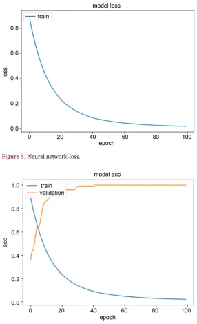
As shown in Table 4 and Table 5, we can conclude that adding layers in-creases accuracy. Figure 5 and Figure 6 depict Table 5.

5.1.3. Autoencoder (Encoding_Dim = 2, Activation = “Relu”, Optimizer = “Adam”, Lose = “Mse”)

As shown in Table 6, autoencoder with decision tree yields higher accuracy.

5.2. Longitudinal Comparison

As shown in Table 7, neural network with truncate = 100 with added layers with dropout has the highest accuracy. And all the new models have higher accuracy than the old ones.

6. Conclusions

Support vector machine, neural network with dropout, and autoencoder are three relatively new models applied in bankruptcy prediction problems. Their accuracies outperform those of the three older models (robust logistic regres-sion, inductive learning algorithms, genetic algorithms). The improved aspects include the control for overfitting, the improved probability of finding the global maxima, and the ability to handle large feature spaces. This paper compared and concluded the progress of machine leaning models regarding bankruptcy pre-diction, and checked to see the performance of relatively new models in the context of bankruptcy prediction that have rarely been applied in that field.

DOI: 10.4236/jmf.2017.74049 916 Journal of Mathematical Finance

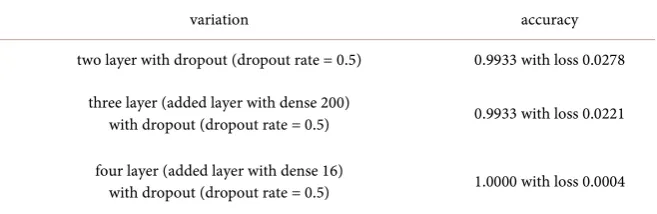
Table 4. Accuracy of Neural Network Model with Two, Three, and Four Layer.

variation accuracy

two layer with dropout (dropout rate = 0.5) 0.9933 with loss 0.0278

three layer (added layer with dense 200)

with dropout (dropout rate = 0.5) 0.9933 with loss 0.0221

four layer (added layer with dense 16)

with dropout (dropout rate = 0.5) 1.0000 with loss 0.0004

Table 5. Accuracy of Neural Network Model with Truncate 50 or 100 and With Four

Layers.

variation accuracy

truncate = 50 with four layers

(added layer dense 16,200) with dropout rate 0.5 0.9950 with loss 0.0389

truncate = 100 with four layers

(added layer dense 16,200) with dropout rate 0.5 1.0000 with loss 0.0004

Table 6. Accuracy of Neural Network Model with SVM or With Decision Tree.

variation accuracy

with SVM 0.9867

with decision tree 0.9933

Table 7. Accuracy of Neural Network Model with Different models.

model accuracy

Robust logistic regression 0.6944

inductive learning algorithms (decision tree) 0.897

genetic algorithms 0.94

neural networks without dropout 0.903

SVM truncate = 100 0.9933

Truncate = 100 with four layers (added layer dense 16,200)

with dropout rate 0.5 1.0000 with loss 0.0004

autoencoder (with decision tree) 0.9933

DOI: 10.4236/jmf.2017.74049 917 Journal of Mathematical Finance

Figure 5. Neural network-loss.

Figure 6. Neural network-accuracy.

when the most relevant information only makes up a small percent of the input. The solutions to overcome these drawbacks are yet to be found.

References

[1] Hauser, R.P. and Booth, D. (2011) Predicting Bankruptcy with Robust Logistic Re-gression. Journal of Data Science, 9, 565-584.

[2] Kim, M.-J. and Han, I. (2003) The Discovery of Experts’ Decision Ruels from Qua-litative Bankruptcy Data Using Genetic Algorithms. Expert Systems with Applica-tion, 25, 637-646,

DOI: 10.4236/jmf.2017.74049 918 Journal of Mathematical Finance

[4] Sirvastava, N., et al. (2014) Dropout: A Simple Way to Prevent Neural Networks from Overfitting. Journal of Machine Learning Research, 15, 1929-1958.

[5] Dev, D. (2017) Deep Learning with Hadoop. Packet Publishing, Birmingham, 52. [6] Nielsen, F. (2001) Neural Networks—Algorithms and Applications.

https://www.mendeley.com/research-papers/neural-networks-algorithms-applicatio ns-5/

[7] Robinson, N. (n.d.) The Disadvantages of Logistic Regression.

http://classroom.synonym.com/disadvantages-logistic-regression-8574447.html

[8] Sima, J. (1998) Introduction to Neural Networks. Technical Report No. 755. [9] Baldi, P. (2012) Autoencoders, Unsupervised Learning, and Deep Architectures.

Journal of Machine Learning Research, 27, 37-50.