Resource allocation for multi sensory virtual environments

(1)

warwick.ac.uk/lib-publications

A Thesis Submitted for the Degree of PhD at the University of Warwick

Permanent WRAP URL:

http://wrap.warwick.ac.uk/92730

Copyright and reuse:

This thesis is made available online and is protected by original copyright.

Please scroll down to view the document itself.

Please refer to the repository record for this item for information to help you to cite it.

Our policy information is available from the repository home page.

(2)

Resource Allocation for Multi-Sensory

Virtual Environments

by

Efstratios Doukakis

Thesis

Submitted to the University of Warwick for the degree of

Doctor of Philosophy

Warwick Manufacturing Group

(3)

(4)

List of Figures

1.1 Examples of multi-sensory virtual environments. . . 1

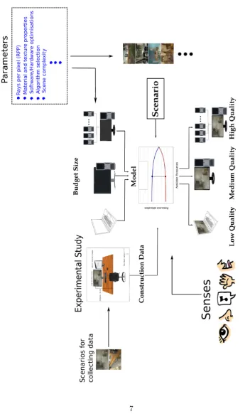
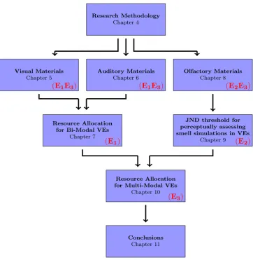
1.2 Research methodology schematic diagram. . . 7

2.1 Physical properties of a sinusoidal wave. . . 15

2.2 Just noticeable di↵erence thresholds for frequency and sound intensity. 18 2.3 Median, horizontal and frontal planes in sound localisation. . . 20

2.4 Example HRTF data from the KEMAR database. . . 22

2.5 Light and Audio wave phenomena. . . 26

3.1 Basic anatomy of the Human Eye. . . 41

3.2 Basic anatomy of the Human Ear. . . 43

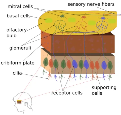
3.3 Basic anatomy of the human olfactory system. . . 45

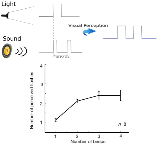
3.4 The illusory flash e↵ect. . . 53

3.5 Example of a visual saliency map. . . 60

3.6 Example of a waveform, spectogram and an auditory saliency map. . 62

3.7 Pipeline of the VDP computational model. . . 67

4.1 Schematic flow diagram of the thesis chapters. . . 77

5.1 Radiance geometrical definition. . . 85

5.2 Classic Ray tracing. . . 88

5.3 Path tracing. . . 89

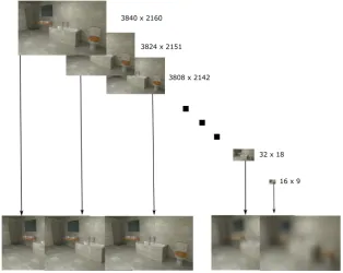
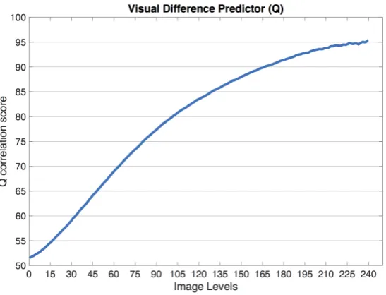
5.4 Images at di↵erent Resolution scales. . . 91

5.5 Average values of the Qcorrelation results across all scenarios. . . . 93

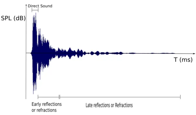
6.1 Waveform of a simulated room impulse response. . . 97

(11)

7.1 Snapshots of the scenarios used inE1 experimental study. . . 110

7.2 Hardware set-up of theE1 experimental study. . . 111

7.3 Snapshots of the experimental software used inE1 experimental study.113 7.4 Descriptive summary of the results of theE1 experimental study. . 115

7.5 Resolution and sampling rate average preferences. . . 118

7.6 Results of the validation study following the experiment E1. . . 124

8.1 Brownian motion for simulating smell di↵usion. . . 128

8.2 Olfactory simulation pipeline using CFD . . . 129

8.3 A polyhedron control volume. . . 130

8.4 Transportiveness property in fluid mechanics problems. . . 138

8.5 Concentration and velocity field for the Bathroom scenario. . . 145

8.6 Concentration and velocity field for the Car scenario. . . 146

8.7 Concentration and velocity field for the Kitchen scenario after 800 sec of simulation. . . 147

8.8 Concentration and velocity field for the Kitti scenario. . . 148

8.9 Boundary conditions set-up of the VEs. . . 149

8.10 Odour concentration results measured in the probe location. . . 150

8.11 Figure of the olfactory display used for the delivery of the smell im-pulses. . . 153

9.1 Stages of an experimental trial of the experimentE2. . . 158

9.2 Snapshot of the experimental software used in theE2 experimental study. . . 161

9.3 Hardware setup of theE2 experimental study. . . 162

9.4 Results of theE2 experimental study. . . 164

10.1 Smell source locations of the scenarios used in theE3 experimental study. . . 173

10.2 Hardware set-up of theE3 experimental study. . . 174

10.3 Snapshots of the software used in E3 experimental study. . . 175

10.4 Proportion of times the smell impulse was set ON. . . 178

10.5 Mean allocation percentages and confidence intervals for graphics and acoustics. . . 181

10.6 Results of the validation study following the experiment E3 for the Car scenario (graphics/acoustics). . . 188

(12)

10.8 Results of the validation study following the experiment E3 for the Kitchen scenario (graphics/acoustics). . . 190 10.9 Results of the validation study following the experiment E3 for the

Kitchen scenario (smell) . . . 191 10.10Results of the validation study following the experiment E3 for the

Kitti scenario (graphics/acoustics). . . 192 10.11Results of the validation study following the experiment E3 for the

Kitti scenario (smell) . . . 193

(13)

List of Tables

7.1 Theoretical budgets used in E1 experimental study. . . 108

7.2 Contrast comparisons between budgets. . . 116

7.3 Contrast comparisons between scenarios. . . 117

7.4 Regression coefficient estimates for models ME1₁ andME1₂ . . . 120

8.1 Physical computation times for di↵erent mesh discretisation levels. . 151

9.1 Model comparisons using deviance criterion. . . 165

10.1 Theoretical costs for smell impulses. . . 171

10.2 Contrast comparisons for proportions between budgets. . . 179

10.3 Contrast comparisons for proportions between scenarios. . . 179

10.4 Contrast comparisons between budgets and scenarios for graphics. . 182

10.5 Contrast comparisons between budgets and scenarios for acoustics. . 182

10.6 Least squares regression estimates of the multivariate model ME1₁ . . 184

10.7 Coefficients of determination for the multivariate model ME3 1 . . . 184

10.8 Least squares regression estimates of the multivariate model ME3₂ . . 185

(14)

Acknowledgments

I would like to express my sincere gratitude to all those who gave me the possibility

to complete this thesis. First of all, my supervisors Kurt and Alan. Both of them

gave me guidance and courage to keep going while they supported my application for

extra funding towards the end of my PhD. Saying “thank you” is an understatement.

I would like also to thank the research fellows of the visualisation group.

Carlo and Tom were always eager to provide assistance to every PhD student without

even being asked to do so. I am also very lucky for meeting and spending time with

Rosella, Debmalya, Ali, Pinar, Jon, Amar, Josh, Tim and Emmanuel. Thanks for

everything. Ratnajit, thanks for the stimulating discussions and the fun we have

had the last four years. I was very fortunate to come across many people during

this PhD. Doctor Andrew Garmory and Professor Martin Passmore helped me a lot

with my odour transport simulations during my visits to Loughborough university.

Ahmed al Makky, who inspired me to get started with OpenFoam and implement

turbulence modelling in my simulations. I would like also to thank Doctor Derrick

Watson for our discussions about psychophysics procedures. Many of the ideas

presented in chapter 9 have come about due to discussions with him. Many thanks

also to my examiners, Professor Caroline Meyer of Warwick University and Doctor

Kirsten Cater of Bristol University for making the viva very pleasant.

I would like to thank my parents and sister for their motivation and

encour-agement. Joanna, I would not have made this without your love and support. This

(15)

Declarations

Peer-reviewed journal papers:

• Doukakis E., Debattista K., Bashford-Rogers T., Harvey C., Chalmers A.: Audio-Visual Resource Allocation for Bi-Modal Virtual Environments,

Com-puter Graphics Forum. (conditionally accepted) 2016.

(16)

Abstract

Fidelity is of key importance if virtual environments are to be used as au-thentic representations of real life scenarios. However, simulating the multitude of senses that comprise the human sensory system is a computationally challeng-ing task. With limited computational resources it is essential to distribute these carefully in order to simulate the most ideal perceptual experience for the user.

This thesis investigates this balance of resources across multiple scenarios where combined audio, visual and olfactory cues are delivered to the user. Starting with bi-modal virtual environments where audio and visual stimuli are delivered to the users, a subjective experimental study, denoted as E1, was undertaken where participants (N = 35) allocated five fixed resource budgets for adjusting the quality of the displayed graphics and acoustics stimuli. In this experiment, increasing the quality of one of the sensory stimuli decreased the quality of the other. Findings demonstrate that participants allocate more resources to graphics, however as the computational budget is increased the allocation ratio between graphics and acous-tics decreases significantly. Based on the results, an audio-visual quality prediction model is proposed and successfully validated against previously untested budgets and scenarios.

The introduction of realistic olfactory stimuli is considered necessary if multi-sensory virtual environments are to be used as genuine representations of real life experiences. The estimation and delivery of smell impulses includes many challenges and significantly di↵ers from the methods used for computing and displaying au-ditory and visual cues. Furthermore, the absence of a quality metric for assessing olfactory stimuli makes the introduction of an olfactory quality scale in the resource allocation framework significantly challenging.

(17)

accu-rate smell transport simulations. This outcome enables computational savings from avoiding exhaustive smell transport simulations that provide no perceptual benefit to the user.

Having considered the limitations associated with assessing smell impulses in terms of quality, a third experimental study is proposed, denoted as E3, and is exploited for resource allocation in tri-modal virtual environments. The experimen-tal layout of E3 (N = 25) builds on the framework proposed inE1 including the delivery of physically accurate smell impulses to the user. The display of the smell bursts is implemented in a binary fashion (two levels or ON/OFF smell) along with the quality levels for the senses of vision and hearing as selected in E1. The smell concentration level presented in this experiment follows from the results of the JND threshold estimation for odour concentration presented in the psychophysics study

E2.

In conclusion, the research presented, shows that human preference criteria can be fully exploited in the design and delivery of multi-sensory virtual experiences. Experimental data can be used to derive computationally inexpensive prediction models that direct resource allocation in rendering pipelines where diverse sensory stimuli are simulated and delivered to the users.

(18)

Chapter 1

Introduction

Virtual Environments (VEs) provide the opportunity to simulate a wide range of applications, from training to entertainment, in a safe and controlled manner. VEs intend to provide the experience of being in a real place where interaction with ob-jects or characters is possible. A primary challenge of VEs is to provide realistic rep-resentations of real world environments. For applications which require high levels of authenticity, the VEs need to provide multiple, physically accurate sensory stimuli. The existence of multiple senses in the VE context expands the number of potential applications while it increases the level of immersion [HB96, LVK02]. Examples in-clude, but are not limited to, commercial vehicle simulators [YSYT94, FMT11], video games [RLC+07, GBW+09] and applications in the prognosis and treat-ment of various human disorders in healthcare [Riv03, TS10] and neuropsychol-ogy [RBvdZ+00, Mor04]. Examples of multi-sensory VEs are given in figure 1.1.

Figure 1.1: Examples of multi-sensory virtual environments. Left: Driving simula-tor [PfSI12],Middle:Virtual infirmary [Vir16],Right: Video games [Ger99].

(19)

(e.g. boundaries, objects, etc.) and provide an understanding of its shape, scale and surrounding properties (e.g. surface materials).

Other senses have recently been introduced in bi-modal frameworks as a mean of increasing the level of fidelity and sense of presence in the VEs. Ex-amples in the literature include haptics, feel and smell cues [MC97, HS13]. The significance of the sense of olfaction, in particular, might not be initially obvi-ous, but it a↵ects how humans feel, think and behave in real life. Furthermore, there is evidence that people tend to recall memories associated with a perceived odour [HE96, SP04, PSNG06]. Olfactory cues have only recently been exploited in multi-sensory rendering frameworks either with the objective of reducing the compu-tational complexity of displayed visual stimuli [RCHR07, BCB+09] or for enhancing saliency estimation models under the e↵ect of congruent smell stimuli in the virtual scene [HBRDC11].

The computation and delivery of multi-modal VEs in high fidelity requires significant computing resources. Previous work has shown that humans are not able to attend to all the sensory stimuli at the same time in real life situations [Sto98, TN03a]. Such cross-modal e↵ects have mostly been exploited in bi-modal VEs where, usually combined audio and visual stimuli are delivered to the user. Per-ceptual interactions between the senses have been used to compute and deliver lower quality visual [CCL02, RFWB07, HDAC10] or auditory [TGD04, MBT+07] stimuli without the quality compromise being consciously perceived by the average user. Furthermore, many examples in the literature have shown that the perceived quality of a sensory stimulus can be significantly increased under the synchronous e↵ect of a di↵erent sensory cue. Interactions of this kind have mainly been used to increase the temporal or spatial quality of visuals under the e↵ect of auditory stimulations [MDCT05a, MDCT05b, HAC08, HDAC11].

(20)

1.1 The research problem and its significance

The simulation of various sensory stimuli for computing realistic virtual experiences is still not feasible at interactive rates with the existing algorithms and hardware available today. The demand of VEs in di↵erent areas of academia and industry is continuously increasing and the availability of computing resources in these areas varies. It is necessary, therefore, to exploit the available resources in the best pos-sible way for rendering the sensory cues of the VEs. For this purpose, allocating a large amount of resources, either hardware or software, to the senses that are more important for the perceived fidelity and fewer resources to the senses that do not contribute to the overall perceptual experience is considered crucial.

Multi-sensory rendering pipelines exploit interactions between the senses in order to reduce the rendering times by delivering lower quality stimuli without the users being able to discern any degradation in the quality of the overall experience. However, there is no generic way to quantify the level of this interaction so as to adjust the distribution of the resources to the senses of the VE accordingly. Existing multi-sensory rendering frameworks are solely based in heuristics that have reported and studied in perception literature for reducing the rendering times but no work has looked into quantifying this process formally.

The research problem is firstly approached in the context of two senses, namely sight and hearing. The experimental layout is later extended to accommo-date the delivery of olfactory impulses in a tri-modal VE set-up. The experimental layout can be generalised to any number of di↵erent sensory stimuli for distributing the available resources.

1.2 Overall method

(21)

perceptual experience will be delivered to the user.

Adjusting the quality of the sensory stimuli in the experimental layout is a process that depends on many parameters. For instance, the quality of the rendered images strongly depends on the algorithm selection (ray tracing/rasterized images), complexity of the scene, material selection and many others. All these parameters adjust the quality level and a↵ect the computation times. This thesis proposes a methodology for decoupling the resource allocation problem from these factors by using normalised costs that are independent of the algorithm selection and its parameterisation.

1.3 Research objectives and contributions

The experiments implemented in the context of this thesis have a twofold purpose. Firstly, to investigate whether participants’ subjective preferences for resource al-location follow any trends under the e↵ect of di↵erent budget sizes and scenarios. Secondly, to utilise the experimental data in actual applications by designing pre-diction models capable of estimating the percentage of the total budget that should be devoted to do quality improvements in each sense. As the participants allocate resources depending on the quality of the sensory stimuli, it is important to define quality metrics for every sense of the experimental framework. This thesis considers the challenges associated with the definition of metrics in each of the visual, auditory and olfactory modalities.

The contributions of this thesis can be listed as follows:

• A literature review of the field of perceptually based rendering including the description of the psychological phenomena that characterise the co-existence of multiple sensory stimuli.

• The establishment of a solid experimental methodology for resource allocation in bi-modal VE based on user’s actual preferences.

• The development and validation of a statistical model for estimating audio-visual distribution for an input budget and scenario.

• A methodology for rendering physically accurate visual, auditory and olfactory stimuli in the design and delivery of virtual experiences.

(22)

whether these di↵erences can be used as a representative metric for assessing olfactory impulses.

• An extension of the experimental methodology to accommodate the existence of multiple senses giving as example the inclusion of smell impulses in the resource allocation framework.

• Finally, the development of a new statistical model that can estimate audio-visual allocation and additionally predict whether smell impulses should be delivered to the users.

1.4 Thesis outline

This thesis is organised as follows:

• Chapter 2 provides an introduction to the physical and perceptual properties of light, sound and smell. The chapter also explains the basic methods to deliver visual, auditory and olfactory stimuli to the users. An overview of the basic simulation pipeline for computing the three senses is also given.

• Chapter 3 presents an overview of the human perceptual phenomena that consist of the theoretical background of many selective rendering schemas. The discussion is then directed to perceptual interactions between the senses and the way they can be used to reduce computation times in cross-modal selective rendering frameworks.

• Chapter 4 describes the research methodology of the resource allocation exper-imental studies presented in this thesis. The objectives of the experimentsE1,

E2,E3 and their importance for answering the research question are given.

• Chapter 5 explains the process of computing and assessing visual stimuli in the form of rendered images. These are necessary materials for the implementation of the experimental studiesE1,E3.

• Chapter 6 describes the methodology followed for computing and evaluating audible cues. Auditory stimuli are also part of the software materials used for conducting the studiesE1,E3.

(23)

The obtained data are used in the construction of a statistical model for esti-mating audio-visual resource distribution. The model performance is assessed in a validation experimental study.

• Chapter 8 describes the process followed for simulating and delivering phys-ically accurate smell impulses to the users of a VE. This chapter serves for preparing the olfactory materials needed for conducting the experimental stud-iesE2 and E3.

• Chapter 9 presents a psychophysics experimental study (E2) for estimating the JND threshold for odour intensity. The objective of this study is to in-vestigate whether better spatial discretisation of the computational domain in smell transport simulations is a representative metric of olfactory quality.

• Chapter 10 extends the experimental methodology of resource allocation from bi-modal to multi-modal VEs and demonstrated in a tri-modal set-up with the inclusion of the sense of olfaction along with the other senses. A new experiment (E3) is conducted for capturing participants’ preferences. The experimental data are used in the construction of a statistical model whose performance is tested in a validation study.

• Finally, in chapter 11, conclusions and future plans for extending this work are discussed. The contribution of this research in the field of Computer Graphics is also given.

• Appendix A provides the definition of the solid angle used in chapter 5.

• Appendix B provides the basic points of linear and time invariant filters and the process of convolution needed in chapter 6.

(24)

F

igu

re

1.

2:

R

es

ear

ch

m

et

h

o

d

ol

ogy

sc

h

em

at

ic

d

iagr

am

[image:24.595.135.488.171.754.2]

(25)

Chapter 2

Background

This chapter introduces the fundamental properties of light, sound and smell and describes methods to deliver stimuli of these three senses. The basic terminology and concepts of this chapter are necessary for understanding the rest of this thesis.

2.1 Introduction to light

Light can be described either as a bundle of photons (corpuscular theory) or as an electromagnetic wave (wave theory). Electromagnetic waves are composed of an electric and magnetic field that fluctuate together and form a propagating wave which carry energy from one point to another. Every electromagnetic wave has a frequency f, a propagation speed u and a wavelength which are connected by the equation u = f˙ . The wave nature of light was used to explain macroscopic

phenomena such as reflection, refraction, di↵raction and interference [HRW13].

2.1.1 Physical properties of light

Speed of light

(26)

light. The speed of light in this case can be found using:

u= _p1

✏0µ0

, (2.1)

where µ0 is the magnetic permeability and ✏0 is the electric permittivity of the

material [HZZ01].

Wavelength and frequency

Electromagnetic waves can be classified depending on their wavelength. The elec-tromagnetic spectrum encompasses the whole range of wavelengths from 10 11 cm (gamma rays) up to 103 cm (radio waves). This range contains the region of visible light where the human eye operates and perceives visual stimuli. The visible spec-trum ranges from 380 nm up to 750 nm1 or in terms of frequency between 4.3_⇥1014 Hz and 7.7⇥1014 Hz. The human eye recognises light wavelengths as di↵erent colours ranging from violet (short wavelength) up to red colour (long wavelength). All the other visible colours exist in between these wavelengths.

Radiometry and photometry

Properties of light can be described either using physical quantities that involve light energy or by quantifying the perceptual impact of these physical quantities to human observers. The former way describes the area ofRadiometry while the latter is the subject ofPhotometry in the field of Optics. Radiometric quantities include physical measurement of light properties and they are used in the description of light transport through a scene using global illumination algorithms [DBB06]. Pho-tometric quantities express the sensitivity of the human eye at di↵erent frequencies of the visible spectrum and their calculation is based on the derivation of the corre-sponding radiometric quantities [SAM09]. Throughout this thesis both radiometric and photometric quantities are used for describing fundamental properties of light.

Intensity of light

The intensity of light coming from a distant source to an object can be generally ap-proximated if the distance between the source and the object is known. Specifically, the intensity of light reaching an object is inversely proportional to the square of the distance between the object and the light source. This idealisation of the light

(27)

intensity estimation does not take into account cases where light can be absorbed or scattered by the surfaces of the environment.

The radiometric quantity used for describing light intensity is known as Ir-radiance and is measured in Watts/m2. Irradiance can be calculated as

E = I

R2, (2.2)

whereI is the intensity of the light source (measured in Watts) andR denotes the distance between the illuminated object and the light source. Light intensity can also be described using photometric quantities (see section 2.1.3).

2.1.2 Perceptual properties of light

Just noticeable di↵erence threshold

A useful definition when studying the perceptual impact of a physical property is that of the Just Noticeable Di↵erence or JND threshold. It expresses the magnitude that needs to be added to a physical stimulus so as the increase to be percep-tually detectable by the average human. JND thresholds can be estimated using psychophysics experiments and cannot be measured directly using scientific instru-ments.

Luminance and contrast

The photometric quantity that is used to measure light intensity is termed Lumi-nance or Brightness and is measured in cd/m2_{. Candela (cd) is the measurement}

unit used to describe how much light is emitted by a light source. Luminance ex-presses how much light is emitted by a light source per unit area or generally what is the amount of light that is absorbed or reflected by a region [WA01]. Contrast is the di↵erence in luminance between an object and its surroundings and is the primary reason humans can visually perceive objects in real life or in a visual display. The JND threshold for contrast has been measured in previous research and found equal to 0.09 cd/m2 [KP09].

(28)

anymore able to resolve the grating pattern. The ability to perceive this alternating pattern for increasing angular frequencies can be encoded using a humanContrast Sensitivity Function (CSF) that shows how contrast perception scales for increasing spatial frequencies in the visual field. CSFs can be estimated using psychophysical experimental studies where people’s ability to detect alternating grading patterns is captured for di↵erent frequencies.

Weber’s law states that the ratio between the JND threshold of any stimulus and its magnitude is constant. Specifically, Weber’s law for contrast can be written in the following form:

L Lb

=k, (2.3)

where L = Lb Lp expresses the di↵erence in luminance between a patch (Lp) and its backround (Lb). A generalisation of Weber’s law was proposed by Fechner in 1870 and expresses the perceived intensity of any stimulus as a function of its physical magnitude.This law can be written as:

S= log(I), (2.4)

whereS is the perceived intensity of any stimulus andI is its physical magnitude. The constant depends on the stimulus under consideration [SAM09].

Colour perception

The human retina absorbs large collections of photons that have di↵erent wave-lengths (or di↵erent energies). The incoming light information is translated into electrical signals that are processed by the Human Visual System (HVS) and per-ceived as colours of di↵erent intensities. The colours of the visible spectrum that have a single wavelength value are termed asSpectral colours. Mixtures of di↵erent wavelength values can result to colours that elicit the same visual perception as a monochromatic spectral colour [Hun04].

(29)

match can be found by using the colour matching functions which result from the colour matching experimental results. The colour matching functions are used to derive tristimulus values, denoted as R, G and B, that encode the HVS’s response to the spectral composition of the incoming light. Using the tristimulus values, any colour C can be written as:

C=RR+GG+BB,

where R, G and B are unity values for red, green and blue. These values give white light when combined. For given colour matching functions, any colour can be described as a set of tristimulus values R, G and B that express the necessary amount from each primary colour in order to perceive the reference colour at the left hand side of the above equation. When a di↵erent set of matching functions are available, the existing set of tristimulus values can be mathematically transformed to another set of values that uses di↵erent primary colours [SAM09]. Transformations between tristimulus values can be inverted and/or applied collectively depending on the application.

The matching functions that correspond to the RGB tristimulus values can also get negative values. As it is not feasible to add negative light values the amount of light that needs to be subtracted is simply added to the target colour i.e. the one that the three tristimulus values represent. The CIE developed a set of positive matching functions with a new set of associated tristimulus values namely, X,Y and Z. These tristimulus values are organised such that the Y channel represents the luminance of the target colour. It is worth noting that these tristimulus values correspond to primary colours that cannot be visualised as was the case with the primary colours that correspond to the RGB tristimulus values [Gue90].

(30)

2.1.3 Visual display methods

This section summarises the imagery display technologies that are frequently used to display visual stimuli. The luminance range of the visual display is used for dis-tinguishing between Low Dynamic Range (LDR) and High Dynamic Range (HDR) displays.

Dynamic range

Dynamic Range is the ratio of the lowest and highest measurable light intensities in an image or video. In real life the term can either be used to describe human’s eye ability to see from very dark to very bright light conditions or it can be used to describe the level a display monitor (or a capture device) is capable of representing true black or white colours.

In Low Dynamic Range (LDR) every pixel contains an 8-bit value for every one of the Red, Green and Blue channels resulting to a 24-bit true colour infor-mation or approximately a range of 16.7 million colours that can be represented in a traditional display. In many cases 32-bits are reserved for a pixel and these are allocated as 24-bits true colour and 8-bit for alpha transparency. Typical LCD monitors have around 250-300 cd/m2 while the luminance of an LCD television is usually between 300-600 cd/m2_{. This quantity is usually higher for plasma displays}

and LED LCD TVs (around 1000 cd/m2). Higher levels of luminance means that the device is capable of displaying more vivid colours as well as enhanced levels of brightness.

The human eye is a sensitive organ that can perceive a very large luminance range depending on observer’s adaptation to the ambient conditions. Specifically, in very dark surroundings the human eye can perceive luminance levels as low as 0.001 cd/m2 which is the lower limit of the Scotopic vision regime. This threshold has been quantified as the ability of an observer to see a candle at 30 miles on a clear night. It corresponds, on average, at around 90 photons falling at the cornea or 9 photons at the retina [Wal02]. The upper limit of the luminance range is approximately 104 _cd/m2 _{and is achieved under bright daylight conditions. This}

threshold defines the higher end of the Photopic vision regime where vision acuity and perception of colours are both at high levels.

(31)

eye needs time to adapt to the new illumination conditions and the adaptation time depends on whether the transition is from a bright to a dark environment (dark adaptation) or the other way around (light adaptation) [AR96].

High dynamic range imagery takes into account a higher dynamic range aiming to approximate HVS’s luminosity range. An HDR image is either composed of a series of LDR images at di↵erent exposures that contain subregions of the dynamic range or it results as a computer rendered image. As an HDR image contains a wider range of light information, its capture, representation to a display and storage follow more advanced techniques compared to those used in LDR images.

2.2 Introduction to sound

This section describes the main physical properties of sound as well as how humans perceive sound stimuli in an environment. Sound waves are created as pressure vibrations of a medium [Gle15] and can be digitally represented as amplitude values over time (waveform representation).

2.2.1 Physical properties of sound

In contrast to light, sound cannot travel through the vacuum and a medium (solid, gas or liquid) is necessary for the propagation of the sound waves. Through solids sound propagates as a transverse wave; that is a wave whose oscillations are perpen-dicular to the direction of propagation. In liquids and gases, sound propagates in the form of a longitudinal wave, these waves oscillate in the direction of propagation. The speed of sound in a medium depends on its density and its elastic prop-erties. The elasticity of a medium expresses medium’s ability to retain its shape due to external forces that are applied upon it. The Newton-Laplace equation [BK15] can be used to calculate the speed of sound through a medium as:

c=

s

K

⇢, (2.5)

(32)

In gases the speed of sound depends on the temperature. For example, the speed of sound in air under a range of temperatures (from 35 C to 35 C) can be calculated as:

cair= 331.3

r

1 + T

273.15 (2.6)

whereT is the temperature measured in Celsius degrees. At room temperature of 20 C the above formula gives that the speed of sound in air iscair = 343.2 m/s.

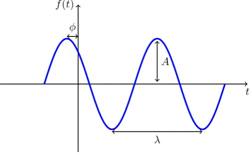
Joseph Fourier in 1827 demonstrated that any periodic waveform can be written as a series of sinusoidal waves of di↵erent frequencies which are integer multiples of a fundamental frequency [Fou27]. For example, the middle C (261.6 Hz) note played in the guitar can be written as a sum of sinusoids at frequencies of 261.6 Hz, 523.2 Hz, 784.8 Hz and so on. A sinusoidal wave is a simpler way to represent a sound wave and can be written in the form:

f(t) =Acos(!t+ ), (2.7)

whereAis the amplitude of the wave,!is its angular frequency measured in rad/sec and is its phase measured in radians. The angular frequency is given as!= 2_T⇡ = 2⇡f whereT is the time of one period andf is the frequency of the sinusoid in Hz. As was the case with light, the frequency and speed of a sound wave are connected as:

= c

f, (2.8)

where denotes the wavelength of the sinusoid. Image 2.1 shows pictorially the physical quantities of a sinusoidal wave.

t f(t)

[image:32.595.194.446.513.667.2]

A

(33)

At standard temperature and pressure conditions (T = 20 C and P = 101.325 kPa [NIS01]) the range of audible wavelengths starts from 0.01715m up to 17.15m. In terms of frequency the audible spectrum is between 20 Hz to 20 kHz and it is usually divided into smaller subregions known as Octave bands. Every octave band contains a centre frequency that is the representative of the band and is used to calculate the lower and upper bounds of the band. The seventh octave band centre frequency is defined as f7 = 1000 Hz and can be used to derive the centre

frequencies of the other bands using the formula: fn 1 = f₂n forn= 2,· · · ,11. The

lower and upper bound of each band can be given by the formulae:

f_nlow= _pfn 2 and f

high

n =

p

2fn. (2.9)

The bandwidth of each octave band is constant and approximately equal to 70.7%.

Sound intensity and pressure

Sound intensity, denoted asI, describes the sound power per unit area. The power that is released from a sound source or received to a surface can be measured in Watts, therefore, sound intensity is measured in Watt/m2_{. Sound pressure, denoted}

asp, expresses the oscillation of a medium’s molecules due to the e↵ect of a sound wave on them. Sound pressure can be measured at any point using microphones which contain sensitive diaphragms that oscillate when triggered by the incoming sound wave. The microphone samples the sound wave and a digital signal that represents the waveform of the sound is created. Sound pressure is measured in N/m2 _{or Pascals.}

Sound intensity and pressure are related to each other and specifically inten-sity is proportional to the square of the pressure [BS04]:

I _/p2. (2.10)

Sound intensity and pressure both fade according to the inverse distance law. The inverse distance law can be stated in terms of pressure at two di↵erent measurement points as:

p2

p1

= r1

r2

, (2.11)

wherer1, r2 are the distances of two points away from the sound source and p1, p2

are their corresponding pressures.

(34)

material. When a sound wave interacts with the environment a portion of the acoustic energy is transmitted into the surface while the rest of it is absorbed or reflected back in the environment. The amount of absorbed acoustic energy depends on the absorption coefficienta(f) of the material and expresses the ratio between the absorbed and incident acoustic energies. The valuea(f) depends on the frequency of the impingent sound and it ranges between 0 and 1 where the value 1 is attributed to a material that absorbs all the incident acoustic energy while 0 indicates that all the incident acoustic energy is reflected. Tabulated absorption coefficient data can be found for various materials and across all the frequency octave bands.

2.2.2 Perceptual Properties of sound

The hearing dynamic range, in terms of sound intensity units, starts fromI0 = 10 12

W/m2 up to Imax= 10 W/m2. I0 is the lowest intensity of a pure tone at 1000 Hz

that can be perceived by a human listener and is known as the threshold of hearing.

Imaxis the highest audio intensity that can be tolerated by a human listener and is

known as the threshold of pain. This vast range can be compactly measured using logarithmic values of the ratio _II

0 as follows:

I(dB) = 10 log₁₀

✓

I I0

◆

, (2.12)

where dB is the shorthand notation fordecibels. The advantage of measuring sound intensity relative to the threshold of hearing I0 is that the wide range of sound

intensities can be measured as the range of 0 to 130 dB where 0 dB is the threshold of hearing and 130 dB is the threshold of pain. This transform is intuitively related to the way human perception works as the perceived intensity of a stimulus changes logarithmically when its physical magnitude increases.

The same relative measurement method can also be used for sound pressure. In that case, the threshold of hearing can be written as p0 = 2·10 5 Newton/m2

and any other pressure level can be calculated in dB as:

p(dB) = 10 log₁₀

✓

p2

p2 0

◆

= 20 log₁₀

✓

p p0

◆

, (2.13)

Equations 2.12 and 2.13 are equivalent as the sound intensity is proportional to the square of the pressure (see formula 2.10).

(35)

to sound intensity via Steven’s law:

L=kIa, (2.14)

where L is the loudness measured in sones, I is the sound intensity, k is a pro-portionality constant that depends on the measurement units andais a parameter that depends on the sensory stimulus measured (e.g. loudness, brightness, contrast, taste, etc.). One sone is the loudness unit for a 1000 Hz sound at intensity of 40 dB. Pitch is connected to the fundamental frequency of a tone (see section 2.2.1) and expresses how bass or tremble a sound is perceived. Pitch is measured in cents and there are 1200 cents in every octave band.

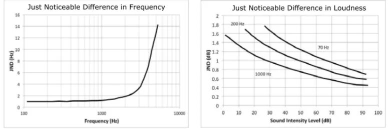
Figure 2.2 (left) shows how the JND threshold for frequency scales for sounds of low and medium frequencies. At low frequencies the average human listener can easily perceive a pair of sounds as di↵erent as the JND threshold is low (approxi-mately 1 Hz). At higher frequencies the JND threshold increases and perceptually distinguishing pairs of sounds becomes more difficult. For sound intensity the JND threshold depends on the frequency of the tone and the intensity level. For example, a 60 dB sound at 200 Hz has a JND threshold of around 0.8 dB. This values change for di↵erent frequency sounds. Figure 2.2 (right) shows how the JND threshold scales for di↵erent frequencies and sound intensity levels.

Figure 2.2: Left: Just Noticeable Di↵erence for frequency. Right: Just Noticeable Di↵erence for sound intensity level at frequencies 70Hz, 200Hz and 1000Hz. Material is adopted from [For13] with author’s permission.

2.2.3 Sound localisation

[image:35.595.128.516.446.575.2]

(36)

opposed to the eyes that can capture only a portion of the environment, the human ear is able to collect auditory information from all directions using binaural and

monaural cues. Binaural cues can be either the Inter-aural Time Di↵erence (ITD) or the Inter-aural Level Di↵erence (ILD) between the two ears. ITD is caused due to the extra time needed for the sound wave to travel around the head and arrive at the ear that is physically further from the sound source. ILD, on the other hand, is the result of a phenomenon known as the Shadowing E↵ect [VWVO04]. The human head obstructs a portion of the original acoustic energy so the sound wave has lower amplitude when arriving at the distant ear. The two ears also receive individual monaural cues that contain information on how the sound waveform is a↵ected by the head shape, shoulders, torso and/or other anatomic characteristics before entering the ear.

Inter-aural time di↵erence

Lord Rayleigh’s Duplex theory [Ray07] was the first study which investigated the problem of sound localisation. This theory assumes that the human head is a com-pletely spherical surface and the wave will reach one of the two ears faster than the other depending on the angle of the incoming sound (see Figure 2.3). The ITD is defined as:

ITD = r

c(✓+ sin✓), ⇡

2 ✓

⇡

2, (2.15)

wherecis the speed of sound in air, ris the radius of the head and✓is the azimuth angle of the incoming sound wave. If the sound source is directly ahead, ITD = 0 and there is no time delay while if the source is o↵to one side then ITD_(max)= a_c(⇡₂+ 1) and a time delay of about 0.7 ms is caused for a human head of typical size.

Inter-aural level di↵erence

Duplex theory explains that the bending of the sound wave around the head is also responsible for amplitude di↵erences between the two ears. The ILD has been found to depend not only on the azimuth angle but also on the frequency of the incoming sound wave. At low frequencies the wavelength is long compared to the head di-ameter and the sound pressure that is exerted at the two ears is approximately the same. At high frequencies the wavelength is quite small and the di↵erence in sound pressure between the two ears can be as high as 25 dB. This di↵erence causes the head shadow e↵ect.

(37)

periodic sounds they can be decoded for frequencies lower than 1.5 kHz [Ray07]. At low frequencies the sound wave bends around the head for less than a full circle (2⇡ radians) and the ITD gives meaningful azimuth directional information. At fre-quencies higher than 1.5 kHz where the head size is comparable to the wavelength of sound the ILD dominates in the localisation perception as the ITD cannot provide meaningful directional information due to the multiple bendings of the sound wave around the head. Duplex theory claims that ITD and ILD can provide sufficient sound localisation information for the whole audible spectrum.

Hor izon

tal plan_e Inc

oming sound

Med_ian plan

e Frontal

plane

✓

z

x y

Figure 2.3: Sound waves reach the head at an azimuth angle ✓ and an elevation angle . The image also depicts the Median, Horizontal and Frontal plane that are used for sound localisation. The definitions given in the image are described in the CIPIC HRTF database [ADTA01].

Head related transfer functions

The use of ITD and ILD can provide accurate localisation information when sound is coming at an azimuth angle on the left or right of the listener. In case that the sound signal arrives at an elevation angle either above or below the head (see Figure 2.3), the use of time or level di↵erences leads to an infinite number of points which have the same ITD or ILD. These points are distributed in a cone that extends outwards from the ear and is known as theCone of confusion [Bla96].

(38)

character-istics of the original waveform creating what are known as monaural cues. Monaural cues can be captured and encoded in the form of digital signals as described in the following.

The monaural cues can be captured for the left and right ear in the form of two signals hL(t) and hR(t) that are termed Head Related Impulse Responses (HRIR). The Fourier transform of each one of these signals is known as Head Related Transfer Function (HRTF) and encodes localisation information between the sound source and each one of the two ears. Figure 2.4 shows a graphical representation of an HRIR in time domain at the horizontal and median planes (these planes are given pictorially in Figure 2.3). The convolution of a sound x(t) that emanates from a sound source with each one of the HRIRs yields signalsxL(t) andxR(t) that contain acoustic localisation information for the left and right ear respectively. They can be calculated as follows:

xL(t) =hL(t)⌦x(t) =

Z ₁

0

x(s)hL(t s)ds, for left ear.

xR(t) =hR(t)⌦x(t) =

Z ₁

0

x(s)hR(t s)ds, for right ear.

(2.16)

The above methodology gives localisation information for both elevation and azimuth but assumes that the sound wave does not interact with any other objects or surfaces between the source and the receiver. In real applications sound waves interact with the surfaces of the environment yielding more localisation cues (e.g. reverberation e↵ects). The e↵ect of these cues can be taken into account and added to the source signal by simulating the basic acoustic features of a room before convolving with the HRIRs. The omission of these sound interactions leads to sounds that are perceived unusually close or inside listener’s head meaning that there is no sense of sound externalisation.

Phase dependence

When two sinusoidal waves of the same frequency have the same amplitude and propagation speed (both magnitude and direction), they can be combined either con-structively or decon-structively depending on their phases. This physical phenomenon is known as wavesuperposition. Specifically, two sinusoidal waves that have the same amplitude A and their phases are 1 and 2 respectively are considered in-phase

when 1 2= 0 for 0 1, 2 <2⇡. In this case the resulting wave sounds louder

(39)

Figure 2.4: Example data from the KEMAR HRTF database [GM94]. Left: Pres-sure that is exerted on the right ear due to a sound source that starts from ahead (✓ = 0 ) and rotates at the horizontal plane. Highest pressure values occur when sound is coming directly from the right (✓ = 90 ) and are depicted with bright colour. When sound comes from the left side (✓= 270 ) the pressure level measured at the right ear is the lowest. Right: Pressure values measured in the median plane. As the sound source moves on the horizontal plane, pressure values do not show the same pattern as previously instead the sound arrival times remain relatively unaf-fected.

waves interfere destructively (out-of-phase waves) and the result is a waveform of 0 amplitude. An example that wave superposition can be frequently noticed is in cinemas or large auditoriums. In this places, sound originates from many di↵erent sources and superposition might lead to silent spots for out-of phase waves or it can act additively, leading to places where sound is unusually loud (sweet spots).

2.2.4 Auditory display methods

(40)

HRTF approximation methods

The calculation of HRTFs is highly dependent on the anatomical characteristics of the listener thus the derivation of an exact transfer function for every individ-ual is not a trivial task. CIPIC [ADTA01] has conducted HRTF measurements in an anechoic environment for many human subjects with di↵erent head anatomical characteristics that represent di↵erent groups of the population. Given the anatomic characteristics of a human listener, someone can choose the best HRTF from the database that matches the specified criteria.

Another way to obtain high quality HRTFs is to measure individual’s anatomic characteristics using head anthropometry measurements as proposed by CIPIC. This method includes various measurements of the pinna (outer ear), head, neck, torso and shoulders and produces an HRTF tailored to the individual that is being mea-sured. This procedure requires a lot of time so it is very difficult to be systematically used by commercial sound systems even though it gives the best possible acoustic experience for the listener being measured.

Many studies [LNL06, SNH+10] propose models that can estimate an HRTF to a certain accuracy. These models include parameters that account for the anatom-ical characteristics of the listener and despite their known limitations give satisfac-tory solutions with little computational cost. A simple HRTF model that can be used for sound localisation in the horizontal plane is the ITD model. This model introduces a time delay at the sound signal that arrives at the two ears depending on the azimuth angle of the incoming wave. The time delay can be calculated as:

TD(✓) =

(

a

c(1 cos✓) if, |✓| ⇡2

a

c(|✓|+22⇡) if, ⇡2 |✓|⇡,

(2.17)

whereais the radius of the head andcis the speed of sound. This model can be implemented in the form of a Finite Impulse Response (FIR) filter and applied to the source signal through convolution. Its application does not provide sound externalisation and elevation cues.

Another HRTF model that can be used for localisation cues in the horizontal plane is the ILD model. This can be implemented as a realizable Infinite Impulse Response (IIR) filter using the following transfer function:

H(s,✓) = f(✓)s+

s+ (2.18)

(41)

transfer function with one pole (root of the denominator) and one zero (root of the nominator) and it enhances the high frequencies when the azimuth angle ✓ is 0 degrees while it fades them when✓ is 180 degrees which is exactly what happens at the head shadowing e↵ect. Similarly to the ITD model, the ILD model cannot simulate the e↵ect of source externalisation and it is not able to provide elevation cues.

Another way to approximate an HRTF is through the combined use of both ITD and ILD models [BR97] and switching between the two depending on the frequency of the incoming sound. This technique overcomes the ambiguity of the ITD model to resolve localisation information for sounds of high frequency. This model still provides localisation information only at the horizontal plane without resolving the sound source externalisation problem.

Brown and Duda proposed an HRTF model [BR97] that includes the com-bined use of the ITD and ILD (formulae 2.17 and 2.18) as a general head model that captures the interaction of the incident sound with listener’s head. They comple-ment the head model with pinnae and shoulder models so as to produce a pair of left and right HRIRs that can capture both elevation ( ) and azimuth (✓) localisation e↵ects. The authors resolve the problem of externalisation by introducing a room echo model which produces room reverberation e↵ects by introducing delays to the signal that is received from the head model. The proposed model can adapt for lis-teners of di↵erent anatomic characteristics through the use of di↵erent parameters for every one of the body models.

Binaural Techniques

(42)

is worth mentioning that if the original sound stream does not contain the e↵ects of the room (i.e. it is an anechoic sound stream), these can be added to it through the use of a Room Impulse Response (RIR) that contains reverberation information specific for an environment. The design and properties of a room impulse response are explained later in section 6.2.

Except from using headphones one can deliver binaural cues through the use of loudspeakers located in front of a listener. This can be done by stopping the sound signal that emanates from the right (or left) loudspeaker to reach the left (or right) ear and is known as crosstalk cancellation [ACB+_{07]. This method can be}

easily applied to a stereo or multi-channel system through the use of Digital Signal Processing techniques (DSP) [RM15].

Binaural techniques are also used for efficient recording of audio in an en-vironment. In that case a head dummy with microphones at each ear is used to capture monaural and binaural localisation cues as a real human head would do.

Monophonic, Stereophonic and Multi-channel Techniques

A simple method to display sound to a listener is through the use of one (Mono-phonic) or two (Stereo(Mono-phonic) audio streams that are delivered using loudspeakers or headphones [Ear89, SE98]. Monophonic sound, as the name indicates, is used for displaying sound that originates from one direction. Stereophonic or stereo are techniques imitate the way ITD and ILD localisation methods work. For a pair of loudspeakers located in front of the listener at the horizontal plane, di↵erent de-lay and gain levels are applied for each of the two signals that are directed to the two loudspeakers. This gives the impression that sound is coming from di↵erent directions in the horizontal plane.

(43)

2.3 Wave phenomena

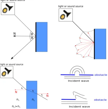
[image:43.595.126.482.201.559.2]

Sound and light are transported in the form of waves. These waves interact with the surfaces of the environment resulting to wave phenomena such us reflection, refraction, di↵raction (see Figure 2.5) and interference.

Figure 2.5: Light and Audio wave phenomena. Top-Left: Reflection,Top-Right:

Scattering,Bottom-Left: Refraction,Bottom-Right: Di↵raction. Images of the physical phenomena were adopted by [HRW13]

Reflection

(44)

the same angle ✓ or it can be di↵use depending on the reflectivity properties and roughness of the incident surface. Reflection also depends on the incident angle and the direction of oscillation of the incoming wave (longitudinal or transverse waves). For light waves, reflection properties can be estimated for various materials using Fresnel’s equations [HZZ01].

Refraction

Refraction is the phenomenon where the direction of an incident wave changes when entering a di↵erent mediumwith di↵erent refraction index. The speed of light in a medium depends on its refraction index and when light enters from a medium of low refraction index (e.g. air) to a medium of higher refraction index (e.g. water) it bends towards the surface’s normal vector. If the two media have refraction indices

n1 and n2, Snell’s law can be used to calculate the angle that the wave propagates

into the medium with the higher refraction index. This is given as:

n1

n2 =

sin✓1

sin✓2 (2.19)

where ✓1 is the incident angle and ✓2 the angle of the refracted wave with the

normal vector N when propagating into the medium with refractive indexn2 (see

Figure 2.5). When light refracts, the wavelength of the incident wave either increases or decreases but its frequency remains constant. This causes the speed of the wave to change accordingly depending on the media that the wave propagates into.

Di↵raction

Sound and light waves can propagate through openings or around barriers that are found on their path. This phenomenon is known as di↵raction. The e↵ects of this phenomenon are more noticeable when the wavelength of the propagating wave is comparable to the geometry size of the object that the wave di↵racts upon (see also Figure 2.5).

Interference

(45)

2.4 Introduction to olfaction

Human perception is based on stimulations coming from multiple senses, namely, vision, hearing, olfactory, gustatory and tactile sensory stimuli. The significance of the sense of smell, in particular, is not initially obvious but it a↵ects how some-one thinks, feels and behaves [SP04, PSNG06]. The sense of olfaction is related to recalling memories associated with a perceived scent, a phenomenon known as

olfactory-evoked memory. This phenomenon is attributed due to the direct link of the olfactory cortex with the limbic system in the human brain. The limbric system is responsible for recalling previous memories or adjusting our emotional state [HE96].

The sense of olfaction has not been given the same merit compared to the other senses that are frequently used in Virtual Reality (VR) applications. This can be mainly explained due to the limited knowledge of the human olfactory system and the way it receives and processes odour stimuli. The human nose can discriminate more than 1 trillion smells using an underlying mechanism that is composed of multiple and diverse olfactory receptors [BMVK14]. The majority of these smells are composed of many di↵erent chemical compounds that cannot be discriminated individually. When their mixture is received by the nose the Human Olfactory System (HOS) perceives them as a single odour. This phenomenon is known as

perceptual blending [LL98] and is quite significant in the sense of olfaction.

Smell perception contains three basic stages which are: estimate the intensity of the smell, qualitatively describe the perceived smell and finally express subjective opinion of how pleasant or not is the perceived smell (hedonic tone) [HCL03]. Smell detection and identification is highly subjective although there are smells that can be identified in concentrations as low as 4_⇥10 15 grams/litre and recognised in concentrations of 2⇥10 13 grams/litre. These measurements represent statistical estimations of the population and are subject to human variability [Nef98, PSNG06]. This section reviews the physical characteristics of odorous molecules and explains the two physical processes that govern smell transport. Following this, a description is given on the how smells are assessed and classified by humans. Finally, the state of the art technology for displaying and analysing odours is presented.

2.4.1 Physical properties of smell

Volatile organic compounds

(46)

pressure at ordinary room temperature conditions. These compounds have a low boiling point which is the reason why large numbers of molecules can evaporate from their liquid or solid form into the ambient air over a period of time (volatility property). There is a large number of VOCs that are inhaled by the human olfac-tory system on a daily basis and many of them are odourless, while others can be toxic when inhaled in large amounts. Health and safety standards report lists of VOCs that can be harmful when received in large concentrations. These standards also propose safe ranges of temperature and pressure in di↵erent places (working environments, hospitals, schools, etc.) as a measure of precaution for preventing faster evaporation rates of these compounds in the ambient air [CEN03].

Odour concentration

When an odour is spread in the environment, it mixes with the air and/or other odours creating a homogeneous mixture (smell-air mixture) [ADP01]. The amount of the odorous substance characterises how diluted or concentrated is the smell in the mixture and can be measured using parts per million (ppm), parts per billion (ppb) (1 ppm = 103 _{ppb) or parts per trillion (ppt) notation (1 ppm = 10}6 _ppt).

This is a relative measure that is frequently used to describe two dimensionless quantities known asmass fraction and molar fraction. Mass fraction is given as:

w= m

mT

(2.20)

where m is the mass of the odour and mT is the mass of the mixture. In mole

fraction the above ratio is expressed in terms ofMoles for both the odour and the mixture instead of masses. Both of these quantities can be used to quantify the amount of odour relative to the amount of the total mixture. For example, 1 ppm of a specific odour (e.g. aroma) means that 1 kg of mixture will contain 1 mg of odour. Measurements in ppm or ppb are practical as they allow to describe concentrations of tiny amounts of odour in large air mixtures.

Di↵usion and convection

The motion of odorous particles can be described through a physical process termed

(47)

or pressure gradients, etc.). The phenomenon of di↵usion is not strictly limited to describe odours movement but it can be generally used to describe the spread of one substance into another when the two substances are either liquids or gases. Similar is the concept of energy di↵usion in the form of heat. Heat disperses from areas of higher temperature to cold regions of a room.

Apart from di↵usion there is one more natural process that accounts for smell transport in a medium and is termed Convection. Convection is the process that describes the bulk transport of fluid mass due to the flow of the fluid in an environment. For example the flow of an air draught through a window can convect a smell plume in a room. In that case the spread of the smell in the environment will be achieved much faster than in the case where the odour is transported in a sealed room through di↵usion.

Convection in an environment can be caused due to di↵erent temperatures or pressures at di↵erent areas of the domain. Using the same example as before, someone can imagine a closed room with a hot radiator in it. The temperature gradient between the hot radiator surface and the cold environment causes large amounts of air to circulate around the room (heat transfer) and disperse a smell plume. Another example, is water flow through a pipe. The application of di↵erent pressures at the two ends of the pipe causes water movement in the direction from higher to lower pressure. The physical phenomena of convection and di↵usion are sometimes collectively termed as Advection depending on the physical context of the problem under consideration.

2.4.2 Perceptual properties of smell

Smell habituation and anosmia

This section describes fundamental properties of the Human Olfactory System (HOS) when interacting with olfactory stimuli at various concentrations. Temporal atten-uation of olfactory perception is a phenomenon that happens in a daily basis even though we might not realise it. Permanent loss of olfactory perception is rare and can be caused due to a damage to the olfactory bulb and/or the brain.