The Study on the Flow Generated by an Array of Four Flettner Rotors: Theory and Experiment

ISSN Online: 2152-7393 ISSN Print: 2152-7385

DOI: 10.4236/am.2017.812132 Dec. 29, 2017 1851 Applied Mathematics

The Study on the Flow Generated by an Array of

Four Flettner Rotors: Theory and Experiment

Fernando Garzón

1

, Aldo Figueroa

2

1_{Instituto de Investigación en Ciencias Básicas y Aplicadas, Universidad Autónoma del Estado de Morelos, Cuernavaca, México} 2_{CONACYT-Centro de Investigación en Ciencias, Universidad Autónoma del Estado de Morelos, Cuernavaca, México}

Abstract

We present an immersed array of four rotors whose promoted flow can be mathematically modeled with a creeping flow solution from the incompressi-ble Navier-Stokes equations. We show that this solution is indeed representa-tive of the two-dimensional experiment and validate such class of solution with experimental data obtained through the Particle Image Velocimetry technique and time-lapsed particles visualizations.

Keywords

Fluid Mechanics, Flettner Rotor, Fundamental Solutions

1. Introduction

Boats ships have crossed the oceans around the globe for centuries by the use of paddling, sails, engine propellers or even turbine propellers. An alternative to the latter propulsion systems is the rotor ship. Through this alternative tech-nique, the ship is propelled, at least in part, by large vertical rotors, sometimes known as rotor sails. German engineer Anton Flettner was the first to build a ship which attempted to tap this force for propulsion, and the ships are some-times known as Flettner ships [1]. A rotor ship is a type of ship designed to use the Magnus effect for propulsion, where the rotation of a solid body can modify its trajectory due to the frictional forces within fluids as consequence of its vis-cosity [2]. Flettner ships have arrays of large rotorsails that rise from its deck which are rotated via a mechanical linkage to the ship’s propellers. Trials con-firm fuel savings of 2.6 percent using a single small Rotor Sail on a route in the North Sea. With these fuel savings, this new wind propulsion technology has a payback period of just four years [3]. Flettner rotor propulsion system presents How to cite this paper: Garzón, F. and

Figueroa, A. (2017) The Study on the Flow Generated by an Array of Four Flettner Rotors: Theory and Experiment. Applied Mathematics, 8, 1851-1858.

https://doi.org/10.4236/am.2017.812132

Received: December 6, 2017 Accepted: December 26, 2017 Published: December 29, 2017

Copyright © 2017 by authors and Scientific Research Publishing Inc. This work is licensed under the Creative Commons Attribution International License (CC BY 4.0).

http://creativecommons.org/licenses/by/4.0/

DOI: 10.4236/am.2017.812132 1852 Applied Mathematics success in reducing fuel consumption and carbon dioxide (CO2) emissions.

Re-cent examples such as Enercon’s E-ship 1 have proven seaworthy and economi-cally viable along major shipping routes [4].

Recently, some preliminary assessments of numerical simulations have been conducted by comparison with experimental investigation of Flettner rotors in order to evaluate the functional relationship and the interaction between the control factors [5], the preliminary design of the Flettner rotor as a ships aux-iliary propulsion system [6], its evaluation with another wind power technology, namely, the towing kite [7], and characterized in terms of lift and drag coeffi-cient [8].

In contrast to the previous studies, in this article, a simple model derived from the Navier-Stokes equations is obtained and compared with a simple experi-mental model that represents the Flettner rotors from the Enercon’s E-Ship 1, with four large rotor sails [9] when the ship is at rest and no flow is incident to it. The objective is the study of the behaviour of the flow patterns due to the rotat-ing cylinders.

2. Statement of the Problem

The theoretical approach begins with the mass and momentum conservation for real fluids [10]

0

∇ ⋅ =u (1)

(

)

1 2

p

t ρ ν

∂

+ ⋅∇ = − ∇ + ∇

∂

u

u u u (2)

where the velocity vector is denoted by u, p is the pressure, ρ is the density,

ν _{is the kinematic viscosity and t represents time. Considering that the surface}

is flat, and that the motions is laminar, thus the motion of the flow occurs on the

x-y plane and the perpendicular velocity is negligible, thus we assume that the flow is two-dimensional. As a first approach, we consider a single rotor. Locating the origin in the geometrical center of the rotor and using polar coordinates, the flow can be considered as symmetric around the origin, that is, independent of the θ_{-direction. Thus the velocity vector is} u=u_θ

( )

r , which automatically sa-tisfies the continuity Equation (1) and the Navier-Stokes Equation (2) for the r

and θ components are

2 1 d d u p r r θ ρ

= ₍₃₎

2 2 d d 0 d d u u r r r

θ ₊  θ₌

 

  (4)

Equation (4) is a homogeneous second order differential equation, thus we must impose two boundary conditions. The first one is that the velocity at infin-ity is zero, that is uθ

( )

∞ =0. The second one is a non-slip condition, as the cy-linder rotates with a uniform angular velocity ω, the tangential velocity at the cylinder’s radius Ri is: uθ

( )

Ri =

ω

Ri, where ω =2πf and f is the rotating

DOI: 10.4236/am.2017.812132 1853 Applied Mathematics

( )

Ri2

u r

r θ

ω

= ₍₅₎

The stream lines can be obtained with the following relation d

dr uθ

ψ

= ₍₆₎

where

ψ

( )

r is the stream function. The boundary condition is

ψ

( )

Ri =0, so we get

( )

2

(

( )

( )

)

ln ln

i i

r R r R

ψ

=

ω

− ₍₇₎

Once the velocity field is known, the pressure distribution can be calculated from Equation (3)

( )

224

2 i R

p r C

r

ρω

= − + ₍₈₎

where C is a constant that can be obtained by evaluating p

( )

∞ . The solution (5) and stream line function (7) in Cartesian coordinates are

( )

2

(

(

)

)

2 2

, Ri cos arctan

u x y y x

x y

ω

=

+ (9)

( )

2

(

(

)

)

2 2

, Ri sin arctan

v x y y x

x y

ω

=

+ (10)

(

_,

)

2

(

_ln

(

2 2

)

_ln

( )

)

i i

x y R x y R

ψ =ω + − ₍₁₁₎

As stated previously, Equations (5) and (7) correspond to single rotor located at the origin. However, as the solution is linear, we can sum the solutions to consider the flow of four rotating cylinders, that is we can perform a superposi-tion of rotors. In Cartesian coordinates, the total stream lines solusuperposi-tions Ψ for the four contemplated sets of rotation are as follows:

( )

(

)

(

)

(

)

(

)

( )

(

)

(

)

(

)

(

)

( )

(

)

(

)

(

)

(

)

( )

(

)

(

)

(

)

(

)

1 2 3 4 , , , , , , , , , , , , , , , , , , , ,

x y x a y x y a x a y x y a

x y x a y x y a x a y x y a

x y x a y x y a x a y x y a

x y x a y x y a x a y x y a

ψ ψ ψ ψ

ψ ψ ψ ψ

ψ ψ ψ ψ

ψ ψ ψ ψ

Ψ = + + + + − + −

Ψ = + + + − − + −

Ψ = − + + + − − + −

Ψ = − + − + + − + −

(12)

where the function ψ _{represents the flow generated by a single rotor with}

neg-ative (clockwise) or positive (counter clockwise) rotation depending on its sign, and a is the shifting length from the origin. Next sections show the experimental procedure and the comparison between this theoretical model and the experi-mental measurements.

3. Experimental Procedure

[image:4.595.214.535.75.300.2]

DOI: 10.4236/am.2017.812132 1854 Applied Mathematics (a) (b)

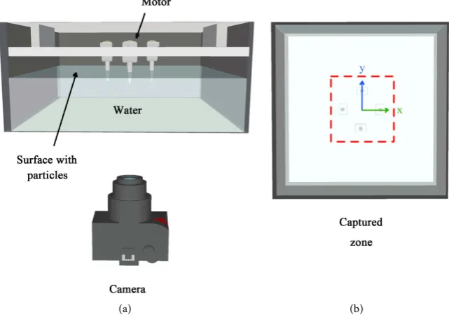
Figure 1. Sketch of the experimental set-up, not drawn to scale. (a) Lateral view; (b) Vi-sualized x-y plane. The flow promoted by the rotors is visualized in the x-y plane tho-rough the PIV technique.

sufficiently far away from the flow. The height of the water level in the glass container is 8 cm. Above the fluid, a rigid table is placed at the top of the box with the four electric DC motors (6 V with gearbox) embedded in it. Consider-ing the geometric center of the rigid table as the origin of coordinates, the elec-tric motors are located at a distance of 2.5 cm from the origin. A rigid cylinder

10 cm

L= is coupled to the shaft of every motor so that the cylinder is partially submerged in the liquid. The radius of every cylinder is Ri =0.4 cm. The DC motors are connected to a power supply whose output voltage is 6 V. As a single cylinder rotates, it promotes a circular fluid flow around itself. The direction of rotation of the cylinders can be changed by inverting the polarity of each motor. As every cylinder rotates independently, four sets of rotation are studied. Every set of rotation produces a different flow pattern. The frequency of rotation of the rotors is f =0.667 Hz. The surface of the fluid is seeded with hollow glass spheres, with an approximated diameter of 10 µ_{m. Images of the surface are} recorded with a photographic camera Nikon D90 with a AF micro-nikkor 60mm f/2.8D lens placed underneath the glass box. Streamlines of the flow cases are obtained by using an exposition time of 30 s. The Particle Image Velocimetry (PIV) technique was used in order to obtain velocity vector fields. The experi-mental data gathered was used to perform a comparative with the theoretical results.

4. Main Results

DOI: 10.4236/am.2017.812132 1855 Applied Mathematics

(a) (b)

[image:5.595.248.498.64.344.2]

(c) (d)

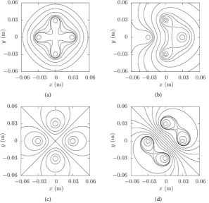
Figure 2. Stream lines of the flows generated by the four sets of rotation. As defined in Equation (12): (a) Set of rotation 1; (b) Set of rotation 2; (c) Set of rotation 3; (d) Set of rotation 4. Experimental results.

(a) (b)

(c) (d)

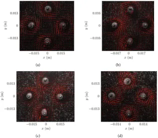
[image:5.595.215.533.402.679.2]

DOI: 10.4236/am.2017.812132 1856 Applied Mathematics the experimental stream lines and the vector fields, respectively, for the four sets of rotation. The stream lines allow to easily identify the flow patterns. The first case, Figure 2(a), is characterized by a squared inner vortex among the four ro-tors sharing a horseshoe at every corner. The second case, Figure 2(b), is an asymmetric flow with two horseshoe patterns. Whereas the third case, Figure 2(c), is a large horseshoe pattern in the geometrical centre. Finally, the fourth case, Figure 2(d), is a jet flow from low-right corner to top-left corner. In turn, the vectorial fields allow us to identify the direction of the flows and their mag-nitude. Moreover, we can appreciate that every cylinder generates a vortex patter around itself and the interaction of the four vortices rotation in different direc-tions produce a global flow. As the theoretical model departs from the latter as-sumption, its predictions are close to the experimental results as seen in Figure 4, where the stream lines from Equation (12) are shown with a=25 mm. Com-paring with Figure 2, only the first case does not agree completely, since the in-ner squared vortex is dismissed by the analytical solution. However, for the rest of the cases the location of the horseshoes, the vortices and the jets are com-pletely predicted. Even more, Figure 5 compares the experimental velocity pro-files with the theoretical predictions from Equation (9) for flow cases 1 and 4, see Equation (12). This is a more detailed comparison and even at this level the qua-litative comparison is very good. The Reynolds number for the experiments

(a) (b)

[image:6.595.227.525.389.677.2]

(c) (d)

DOI: 10.4236/am.2017.812132 1857 Applied Mathematics

(a) (b)

[image:7.595.218.533.62.320.2]

(c) (d)

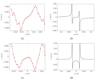
Figure 5. Horizontal velocity u as a function of the y-direction. (a) and (c) experimental profiles of the sets of rotation 1 and 4, respectively; (b) and (d) theoretical profiles of the sets of rotation 1 and 4, respectively.

is Re=URi ν =8, where U is the maximum velocity in the flow field, which demonstrates that the flow regime is laminar and can be compared with the theoretical model. The theoretical predictions are one order of magnitude higher than experimental measurements. This can be attributed to the friction of the container’s bottom with the fluid. Since the model is two-dimensional this fric-tion is not taken into account, thus the velocity in the theoretical model is higher than the experimental obtained through PIV.

5. Conclusions and Suggestions

A solution for the incompressible Navier-Stokes equations was derived in the creeping regime for the case of a single rotation rotor. Considering its linearity, it was superposed to consider an array of four rotors in an unbounded domain. An investigation of the validity of this solution was carried out experimentally. It turned out that this solution represents qualitatively the experimental problem. A verification was established through PIV and time-lapse particles visualiza-tion.

Acknowledgements

This research was supported by CONACYT, Mexico, under project 258623. A.F. thanks the Cátedras program from CONACYT.

References

DOI: 10.4236/am.2017.812132 1858 Applied Mathematics

https://doi.org/10.1036/1097-8542.YB130204

[2] Miller, F.P., Vandome, A.F. and John, M.B. (2010) Magnus Effect.

https://books.google.com.mx/books?id=SAPIXwAACAAJ

[3] Marks, H. and Wachtel, B. (2015) Ship Efficiency Technologies Ready to Set Sail.

https://www.greenbiz.com/article/ship-efficiency-technologies-ready-set-sail

[4] Searcy, T. (2017) Harnessing the Wind: A Case Study of Applying Flettner Rotor Technology to Achieve Fuel and Cost Savings for Fiji’s Domestic Shipping Industry.

Marine Policy, 86, 164-172. https://doi.org/10.1016/j.marpol.2017.09.020

[5] De Marco, A., Mancini, S., Pensa, C., Scognamiglio, R. and Vitiello, L. (2015) Ma-rine Application of Flettner Rotors: Numerical Study on a Systematic Variation of Geometric Factor. VI International Conference on Computational Methods in Ma-rine Engineering, Rome, 1-12.

[6] De Marco, A., Mancini, S., Pensa, C., Calise, G. and De Luca, F. (2016) Flettner Ro-tor Concept for Marine Applications: A Systematic Study. International Journal of Rotating Machinery, 2016, 1-12. https://doi.org/10.1155/2016/3458750

[7] Traut, M., Gilbert, P., Walsh, C., Bows, A., Filippone, A., Stansby, P. and Wood, R. (2013) Propulsive Power Contribution of a Kite and a Flettner Rotor on Selected Shipping Routes. Applied Energy, 13, 362-372.

[8] Gadkari, M., Deshpande, V., Mahulkar, S., Khushalani, V., Pardhi, S. and Kedar, A.P. (2017) To Study Magnus Effect on Flettner Rotor. International Research Journal of Engineering and Technology, 4, 1597-1601.

[9] Wikipedia (2017) E-Ship 1. https://en.wikipedia.org/wiki/E-Ship1