Classification of Event-Related Google Alerts Using
Machine Learning
Wim Kamerman
University of Twente P.O. Box 217, 7500AE EnschedeThe Netherlands
[email protected]
ABSTRACT
DDoS attacks form a severe threat to organizations, as their services can be made unavailable at any moment, resulting in major direct and indirect damage. This re-search compares the performance of 8 supervised machine learning classifiers on a DDoS Google Alert dataset. We provide an annotated dataset and suggest that the Sup-port Vector Machine and the Neural Network perform best based on the desired performance focus. Last, we publish a tool that eases the process of comparing and optimizing multiple (supervised) classifiers on a given dataset, while ensuring valid results. The research can be used to collect all reported DDoS attacks on the internet. This collec-tion can be used to gain a better understanding of DDoS attacks.
Keywords
Machine Learning, Google Alerts, Classification, DDoS
1.
INTRODUCTION
Distributed Denial of Service attacks, better known as DDoS attacks, are attempts to make services or infras-tructure unavailable by flooding them with requests from multiple sources. In 2016, a botnet with more than a mil-lion devices was used to attack DNS provider Dyn. Not only were major services like Netflix and Airbnb unavail-able, access to public broadcasting services like the BBC was also cut off. This shows the major damage DDoS attacks can affect.
DDoS attacks are the most common network security threat experienced by Enterprises, Governments and Educational bodies, while the customers of Service Providers (e.g. ISPs and Data Centers) remain to be the number one target of DDoS attacks [3]. Santanna et al. pointed out that DDoS attacks are easy to execute with DDoS-as-a-Service Providers, even for people without any technical knowl-edge [23].
Much about DDoS attacks has been researched, including how to efficiently detect and mitigate them [29, 15, 16]. Various sources have been used to identify DDoS attacks, including leaked booter databases and DNS provider data. In this research, we explore the possibility to use Google
Permission to make digital or hard copies of all or part of this work for personal or classroom use is granted without fee provided that copies are not made or distributed for profit or commercial advantage and that copies bear this notice and the full citation on the first page. To copy oth-erwise, or republish, to post on servers or to redistribute to lists, requires prior specific permission and/or a fee.
29thTwente Student Conference on ITJuly 6th, 2018, Enschede, The Netherlands.
Copyright2018, University of Twente, Faculty of Electrical Engineer-ing, Mathematics and Computer Science.
Alerts as an additional source to identify DDoS attacks.
Google Alerts is a content change detection and notifica-tion service [28], notifying users when a new or changed result has been detected on a certain keyword. We use a dataset, comprised of Google Alerts, that has been de-scribed by Abhishta et al. [1]. The dataset consists of Google Alerts on the keywords “DDoS” and “Distributed Denial of Service”. This research aims to select the re-sults that describe a DDoS attack. To do this, we classify into four categories: “Attack”,“Arrest”, “Research”and
“Other”. They are defined in Section 3.1.
The main contributions of this paper are:
• An annotated event-related Google Alert dataset
• Comparison of the efficiency of different supervised machine learning classifiers on this dataset
• Suggestion of the best classifier for this specific dataset as a result of the efficiency comparison
• A tool that can help classify a given dataset into various categories
The contributions can be used to collect all reported DDoS attacks on the internet. This information is important to increase our understanding of DDoS attacks, to ultimately outsmart attackers and stop DDoS attacks from happen-ing. Increasing understanding may happen on a wide va-riety of topics. For example, it can be analyzed which attacks get reported and which ones don’t. By correlating the data with other information on DDoS attacks, new insights may be gathered. We might, for example, gain a better understanding of the impact on individual victims.
This paper is structured as follows: first, we will describe the dataset we have used. Second, we will explain the clas-sification methodology in detail. Then, we will present the results, draw conclusions and discuss future work. Finally, we will introduce the classification tool we used for obtain-ing the results of this research. This tool allows extensive exploration to be performed on a given dataset, result-ing in a valid analysis. The annotated dataset, the tool and all other code used will be published at Github1 after publication.
2.
DATASET
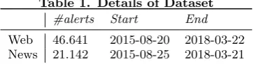
The complete dataset consists of 67.831 alerts, categorized by Google into three categories: web, news and blog. The dataset contains 46.641 web alerts, 21.142 news alerts and 48 blog alerts. Since the number of blog alerts is not sufficient for reliable training and testing, we leave them
Table 1. Details of Dataset
#alerts Start End
Web 46.641 2015-08-20 2018-03-22 News 21.142 2015-08-25 2018-03-21
out. The category “News” is assigned by Google when the source is recognized by Google as being a publisher [11]. The remaining dataset, consisting of only news and web alerts, is summarized in Table 1.
Each Google Alert consists of a title and a short text snip-pet (215±63 characters), a date and a link to the acces-sory page. Additionally, an abovementioned predefined category is present.
3.
METHODOLOGY
We manually annotate a part of the dataset into 4 classes (Section 3.1), followed by automatic classification using supervised machine learning algorithms (Section 3.2).
3.1
Annotation into 4 classes
We manually annotated 1000 Google Alerts into one and only one of the following categories:
1. Attack: describes an occurrence of a DDoS attack.
For example: “Dutch tax office, banks hit by DDoS cyber attacks (...)”
2. Arrest: describes law enforcement after an
occur-rence of a DDoS attack. This includes the identifica-tion of the hacker and responsibility claims. For ex-ample:“Two Israeli teens arrested for running major DDoS service”,“Teenage hacker arrested for unleash-ing DDoS on 911 system”and“British Hacker Ad-mits Using Mirai Botnet to DDoS Deutsche Telekom”
3. Research: an alert describing DDoS research or a
DDoS background article. This includes guides on how to protect against DDoS attacks but does not include DDoS protection service providers. DDoS at-tacks may be described, usually as a reason to write an article, but the main article must not solely be about this particular attack.
4. Other: all other results not fitting in the attack,
arrest or research categories. This includes organi-zations that offer DDoS protection services and com-plaints of gamers accusing DDoS attacks to be the reason for bad gameplay.
The resulting annotated dataset consists of 630 “Web” Alerts and 370 “News” Alerts. It is shown in detail in Fig-ure 1. The arrest category is smallest with 3 web alerts and 14 news alerts.
3.2
Multiclass ML Classification
We have used multiclass Machine Learning classification algorithms. As opposed to unsupervised learning, this type of algorithm is able to learn rules based on not only input but also on output. It requires known labels (the cor-responding correct outputs), so it can learn how to classify based on the targeted output class. We will use the anno-tated classes as output data. We categorize into the four beforementioned classes, so we need to use multiclass al-gorithms, able to distinguish between more than 2 classes.
Attack Arrest Research Other
0% 10% 20% 30% 40% 50% 60% 70%
Number of Google Alerts
14%
0%
18%
67%
25%
3%
36%
33%
18%
1%
25%
54% Web
[image:2.595.79.261.65.111.2]News Combined
Figure 1. Annotated Dataset
3.2.1
Used Algorithms
Kotsiantis [14] has described the best-known supervised machine learning classifiers in detail. He categorized the algorithms into 6 categories: Decision Trees, Neural Net-works, Naive Bayes, k-Nearest Neighbors, Support Vector Machines and Rule Learners. We have compared algo-rithms from all categories, except k-Nearest Neighbors and Rule Learners. k-Nearest Neighbors was left out because of its intolerance of noise, its preference towards classes with more instances and because of its large computa-tional time needed for classification. Rule Learners were left out because they cannot be easily used as incremental learners [14].
We have used the following 9 multiclass supervised algo-rithms from the remaining four categories:
• Logistic Regression (LR): one of the most widely used algorithms for classification in the industry, per-forming well on linearly separable classes [18]. By default LR is a binary model, that is, only capable of separating two classes. To enable multiclass clas-sification we make use of the One-versus-Rest (OvR) technique.
• Support Vector Machine(SVM): introduced by Cortes and Vapnik, it is designed to maximize the so-called
margin[8]. The margin is defined as the distance be-tween the separating hyperplane (the decision bound-ary) and the training samples that are closest to this hyperplane, which are the so-called support vectors [18]. Models with a maximum margin tend to have a lower generalization error, whereas smaller mar-gins are more prone to overfitting. Overfitting occurs when the generalization a model creates to classify unseen data corresponds to closely to the training data. This results in poor performance, as the model takes the specific characteristics of the training data into account too much. Like LR, we use the OvR technique to enable multiclass classification, as SVM is binary by default.
highest information gain, that is, the question that has most influence on the decided class, is on top. Pruning is performed to limit the size of the tree, thus avoiding overfitting. The implementation we use is binary - meaning that every parent node is split up into two child nodes.
• Random Forest (RF): can be intuitively seen as an ensemble of decision trees, in which a voting system for the most popular class is present. By combining multiple decision trees with the same distribution, each suffering from high variance, the generalization error is decreased and the RF is less susceptible to overfitting [5, 18].
• Extremely Randomized Trees(ET): in short: Extra Tree. It was introduced by Geurts et al. as a varia-tion on the Decision Tree [10]. It randomizes both attribute and cut-point choices when splitting a tree node. The strong point of the ET is, besides a high predictive accuracy, the computational efficiency.
• Three Naive Bayes algorithms: Multinomial Naive Bayes (M-NB), Bernoulli Naive Bayes (B-NB)and Gaussian Naive Bayes (G-NB). Naive Bayes algo-rithms make the strong assumption that each predic-tion variable is independent from the others. In text classification this means that each word is seen as in-dependent from all other words. In practice, Naive Bayes systems can work surprisingly well, even when the conditional independence assumption is not true [21].
The Multinomial, Bernoulli and Gaussian preposi-tions refer to the distribution of the probability a feature belongs to a certain class. The Multinomial Naive Bayes is used for discrete data, so in our case for the total number a certain word appears. The Bernoulli Naive Bayes assumes the feature distribu-tion is binary: a word either exists (1) or not (0). And finally, the Gaussian Naive Bayes assumes a normal distribution, and so is used when features are continuous.
• Multi-layer Perceptron(MLP): a network consisting of multiple layers containing single neurons. Neurons are referred to as ADAptive LInear NEurons (Ada-line), first published in 1960 by Widrow and Hoff. What’s interesting about the Adaline algorithm is that it focuses on minimizing continuous cost func-tions, and updates weights based on a linear acti-vation function. Gradient descent optimization is used to learn the weight coefficients. Part of this gradient descent optimization is the learning tech-nique called backpropagation, introduced by Rumel-hart et al. [20]. We make use of Adam, a simple and computationally efficient algorithm for gradient-based optimization of stochastic objective functions [12].
According to [14], Decision Treestend to perform better for classifying categorical features than Support Vector Machines and Neural Networks. Yet, because this might not be true for our unique dataset, we will test using all these algorithms.
3.2.2
Pre-Processing
Next, before applying the algorithms on the dataset, we performed pre-processing. We removed 285 duplicates, by retaining the oldest alert when multiple alerts have the
same url. Afterwards we have selected only English alerts using langdetect2, a language detection library ported from Google’s language-detection. After removal of 10.521 non-English alerts, 58.572 non-English alerts remain.
From these non-duplicate English alerts, 1000 alerts were randomly selected. Annotation was performed as described in Section 3.1.
Further processing has been performed on the annotated dataset. First, we tokenized and lowercased the alerts. Next, we usedterm frequency-inverse document frequency
(TF-IDF) weighting, as described by Salton and Buckley, for feature extraction [22]. This calculates the importance of terms in a document, and in this case, a category. Chi-Square was used select the most outstanding correlated terms as identified by TF-IDF in each of the categories [25]. We ignored words that appeared in over 50% of all alerts (maximum document frequency = 50%). We assume that these words don’t significantly contribute to correct determination of a certain class. We have taken 50% as an initial max-df and varied this variable to find the opti-mal setting. English stopwords have been ignored as well, using the English stopword dictionary3 by the Glasgow Information Retrieval Group.
Tests have also been performed with applying Stanford Named Entity Recognition (NER) to the Google Alert dataset. Stanford NER labels sequences of words in a text which are the names of things [9]. Using NER, we were able to remove words that were identified as a name (person), organization (Cisco, ING) or a location (Ams-terdam, New York). We compared the performance with and without applying NER to the Google Alerts.
3.2.3
Analysis
To avoid overfitting, we use the stratified k-fold cross-validation method as described by Kohavi [13]. This method splits up the training dataset into k equal size subsets (folds). One fold is kept as validation data, while the other k-1 folds are used for training. The validation process will repeat k times so that every fold will be used as validation data once. The effectiveness is then the average of the k times the process has been repeated. We will stratify the folds “so that they contain approximately the same pro-portions of labels as the original dataset” [13]. This yields better bias and variance estimates, especially in cases of unequal class proportions [7]. In our case, we will vary the number of folds, starting with 4 folds. That means that we will create 4 folds of 250 Google Alerts each, and validate the algorithms with those folds accordingly.
Additionally, we have applied over- and undersampling. As can be seen in Figure 1, the various annotated cat-egories are not equal in size. Especially “Arrest” is ex-tremely small, compared to the others. In other words, we are dealing with a skewed class distribution. According to Weiss et al., “the classifier built from a data set with a highly skewed class distribution generally predicts the more frequently occurring classes much more often than the infrequently occurring classes. This is largely due to the fact that most classifiers are designed to maximize ac-curacy.” [26] Over- and undersampling tackle this problem by either reducing the number of features in the major-ity categories (undersampling) or increasing the number of features in the minority categories (oversampling). We have used oversampling, which appears to be most
suit-2https://pypi.org/project/langdetect/ 3
able for small datasets (<10.000 examples), according to Weiss et al. [26].
To prevent information leakage, we used pipelines and a holdout dataset. Information leakage appears when infor-mation from the test data is used for training the model. This makes the model biased towards the test data, result-ing in a too optimistic performance estimation. Pipelines were used to perform pre-processing solely on training data. Additionally, a part of the dataset was held out, only to be used for final testing, after the model has been trained.
To find the best-fitting hyper-parameters for each of the al-gorithms and pre-processing methods, we have performed hyperparameter optimization. A hyperparameter is a pa-rameter from a prior distribution; it captures the prior belief, before data is observed [19]. For example, we have varied the number of Chi-Square features to be used, and the maximum document frequencies of words. Addition-ally, algorithm-specific parameters have been tuned. Final testing as described in the previous paragraph has been performed using the found optimal set of hyperparame-ters.
Lastly, we have varied the input data based on the assump-tion that the title of a Google Alert can better be used to distinguish target categories, compared to the body of the alert. We have found that articles belonging in the “Back-ground” category use a recent attack as a reason to write the article. Therefore this attack is mentioned in the body, while the title actually tells us that this alert belongs in another category. Tests have been performed that increase the importance of the words in the title, compared to the body.
3.2.4
Performance Measurement
The performance of the algorithms is measured using the F-score, which is based on precision and recall. Precision is the number of positive predictions divided by the total number of positive class values predicted. Recall is the number of positive predictions divided by the number of positive class values in the test data [6]. Because the F-score takes both false positives and false negatives into account, the F-score is a good measure. The algorithm with the highest F-score is considered to be most effective for classifying Google Alerts into several classes.
4.
RESULTS
In this section we will present the outcomes of our clas-sification research. In Section 4.1 we show the results of the stratified fold validation on the four categories, and we show an aggregated confusion matrix. Then, in Sec-tion 4.2, we present outcomes of the various variaSec-tions as described in the Methodology section. In Section 4.3, we suggest the best classifier for this dataset, as a result of the efficiency comparisons in Sections 4.1 and 4.2. Finally, as a sidestep, we show the results of 2-class classification in Section 4.4, distinguishing only Attack alerts.
4.1
Results of Stratified 3-Fold Cross
Vali-dation on the Four Categories
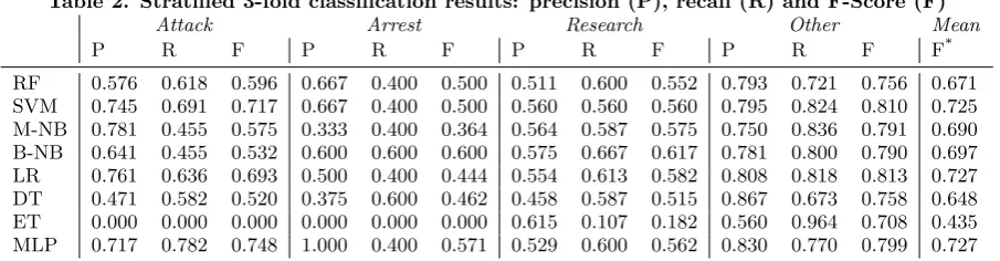
Table 2 shows the results of the various algorithms we tested on the original data. For each algorithm and cat-egory, the Precision, Recall and F-Score are mentioned. The Gaussian Naive Bayes(B-NB)algorithm was dropped from the results because it can only accept continuous data. The sparse matrix that the TF-IDF analysis pro-duces is discrete, and can therefore not be accepted. Con-verting the discrete values to continuous data is possible,
but converting costs a lot of computing power. Therefore, we dropped the algorithm from our analysis.
The Extra Tree Classifier performed exceptionally bad, with a weighted F-Score of 0,435. The reason ET performs so bad is the skewed dataset. With a recall of 0,964 for the Other category, it does not detect any Attack or Arrest alerts. It focuses on the category with most alerts, in this case Other.
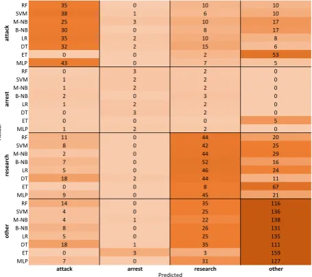
The Arrest and Research columns both have a low F-score on average. The reason for the score in Arrest is simply because the number of samples (17) is too low to get a diverse group of terms for classification. Oversampling for this category has been performed on all algorithms, but still only ∼5 samples could be included in the test subset, resulting in major drops in the score per alert. The Research category suffers from high numbers of alerts being classified as Other, as can be seen in Figure 2.
RF 35 0 10 10
SVM 38 1 6 10
M-NB 25 3 10 17
B-NB 30 0 8 17
LR 35 2 10 8
DT 32 2 15 6
ET 0 0 2 53
MLP 43 0 7 5
RF 0 3 2 0
SVM 1 2 2 0
M-NB 1 2 2 0
B-NB 2 0 3 0
LR 1 2 2 0
DT 0 3 2 0
ET 0 0 0 5
MLP 1 2 2 0
RF 11 0 44 20
SVM 8 0 42 25
M-NB 2 0 44 29
B-NB 7 0 52 16
LR 5 0 46 24
DT 18 2 44 11
ET 0 0 8 67
MLP 9 0 45 21
RF 14 0 35 116
SVM 4 0 25 136
M-NB 4 1 22 138
B-NB 8 0 26 131
LR 5 0 25 135
DT 18 1 35 111
ET 0 3 3 159
MLP 7 0 31 127
attack arrest research other Predicted
attac
k
ar
re
st
res
ea
rch
othe
r
Ac
tu
[image:4.595.312.540.252.454.2]al
Figure 2. Aggregated Confusion Matrix
LR and MLP score best for this dataset, both with a weighted F-score of 0,727. SVM follows closely at 0,725. When comparing these three algorithms, it can be seen that MLP achieves the highest results for Attack (+0,03) and Arrest (+0,07), while only 0,02 lower for Research and 0,01 lower for Other. Weighted though, with Other hav-ing by far the most alerts, it is equal to LR. Not weighted, it performs 0,037 better than LR and 0,023 better than SVM. It can be concluded that MLP performs best for this dataset, as it is able to differentiate better between the different categories.
4.2
Pre-Processing Variations
Table 3 shows 7 variations of the standard data(Std)we used in the first place. The standard data is described in Section 4.1, and the results are shown in Table 2. The weighted F-scores of the standard data are mentioned in the first column of Table 3 as reference. The variations are as follows:
1. NER: Stanford NER was applied to remove named entities from the original Google Alert content.
2. News: Analysis was only performed on the “News” alerts (n=370).
Table 2. Stratified 3-fold classification results: precision (P), recall (R) and F-Score (F)
Attack Arrest Research Other Mean
P R F P R F P R F P R F F*
RF 0.576 0.618 0.596 0.667 0.400 0.500 0.511 0.600 0.552 0.793 0.721 0.756 0.671 SVM 0.745 0.691 0.717 0.667 0.400 0.500 0.560 0.560 0.560 0.795 0.824 0.810 0.725 M-NB 0.781 0.455 0.575 0.333 0.400 0.364 0.564 0.587 0.575 0.750 0.836 0.791 0.690 B-NB 0.641 0.455 0.532 0.600 0.600 0.600 0.575 0.667 0.617 0.781 0.800 0.790 0.697 LR 0.761 0.636 0.693 0.500 0.400 0.444 0.554 0.613 0.582 0.808 0.818 0.813 0.727 DT 0.471 0.582 0.520 0.375 0.600 0.462 0.458 0.587 0.515 0.867 0.673 0.758 0.648 ET 0.000 0.000 0.000 0.000 0.000 0.000 0.615 0.107 0.182 0.560 0.964 0.708 0.435 MLP 0.717 0.782 0.748 1.000 0.400 0.571 0.529 0.600 0.562 0.830 0.770 0.799 0.727
[image:5.595.105.490.218.344.2]*Weighted average of F-Scores
Table 3. F-Scores for various data columns
Std NER News News NER Web Web NER 2xTitle 3xTitle
RF 0.671 0.651 0.507 0.419 0.6912 0.7352 0.655 0.683 SVM 0.725 0.738 0.579 0.605 0.7412 0.7162 0.692 0.713
M-NB 0.690 0.660 0.554 0.527 0.6612 0.6602 0.662 0.651 B-NB 0.697 0.679 0.608 0.612 0.6822 0.6662 0.706 0.693
LR 0.727 0.711 0.5852 0.584 0.6982 0.7072 0.701 0.695
DT 0.648 0.639 0.485 0.468 0.6502 0.6272 0.632 0.625 ET 0.43513 0.4001 0.201124 0.22724 0.62012 0.1212 0.391123 0.3872
MLP 0.727 0.709 0.5932 0.5732 0.7152 0.7252 0.699 0.665
Mean 0.665 0.648 0.514 0.502 0.682 0.620 0.642 0.639
F-Score ofAttack1,Arrest2,Research3orOther4 is 0.000
4. Web: Analysis was only performed on the “Web” alerts (n=630).
5. Web NER: Analysis was performed on the “Web” alerts, after applying Stanford NER.
6. 2x Title: The term document frequencies of the words in the title were doubled.
7. 3x Title: The term document frequencies of the words in the title were tripled.
Analysis on only the News alerts results in low perfor-mance (highest 0,608). We expect this to be a result of the number of samples (n=370) being too low to perform 4-category classification. Only classifying the Web alerts results in higher accuracies: using SVM on the Web alerts even achieves the highest F-Score (0,741). Even though the number of Web alerts (n=630) is higher than the num-ber of News alerts, there are only 3 Web Arrest alerts. This results in no Arrest alerts being detected in the Web alert dataset. In the weighted F-Score however, this is not an issue since the score of 0.000 is only weighed with 3/670, resulting in the high F-score of 0,741.
Applying NER seems to have barely any effect on the re-sults. Only SVM profits from NER for the full dataset (+0,013), while B-NB and ET profit for the News sub-set as well. On the contrary, for the Web alerts, SVM loses 0,025. However, as discussed in the previous para-graph, the Web alerts subset is not suitable for 4-category classification, and can therefore be neglected. It can be concluded that NER only has a consistent positive effect for the SVM.
Analysis on only the title and only the body both resulted in lower F-scores than the title and body combined. This suggests that the title and body reinforce each other. In-creasing the importance of the title in the Google Alerts (2x Title and 3x Title) did not result in higher accuracies than the standard text.
4.3
Suggestion of Best Classifier
According to Kotsiantis, Decision Trees tend to perform better when dealing with categorical features, as opposed to Support Vector Machines and Neural Networks [14]. When we look at the results, though, Kotsiantis was wrong. For all tests, the Decision Trees performed worse than the SVM and the MLP.
[image:5.595.308.544.569.674.2]As can be seen in Table 3, SVM, Logistic Regression and the Neural Network perform best. In Section 4.1 a com-parison was made between these three algorithms on the standard dataset, resulting in the conclusion that MLP is best. However, after analysis of the various other datasets, an even higher score was achieved by the SVM in the NER dataset. The following is a direct comparison between the SVM in the NER dataset (F=0,738) and the MLP in the standard dataset (F=0,727).
Table 4. SVM + NER versus MLP
SVM MLP
P R F P R F
attack 0.632 0.782 0.699 0.717 0.782 0.748 arrest 0.750 0.600 0.667 1.000 0.400 0.571 research 0.580 0.627 0.603 0.529 0.600 0.562 other 0.864 0.770 0.814 0.830 0.770 0.799
avg 0.749 0.733 0.738 0.737 0.723 0.727
Figure 3. 2-class most distinctive terms
4.4
2-class classification
We make a sidestep to show the results of the best per-forming algorithm for a 2-class classification, instead of 4-class. We have merged the Arrest, Research and Other categories into a new “Other” category. This way, only Attack alerts are being distinguished from all other alerts.
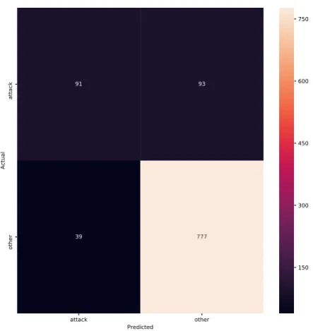
[image:6.595.55.288.51.277.2]Using the same methodology that was used for the 4-class classification, we have found the best performing algo-rithm to be the Support Vector Machine, with the fol-lowing result:
Table 5. SVM 2-class results
P R F
attack 0.700 0.495 0.580 other 0.893 0.952 0.922
avg 0.858 0.868 0.859
Note that the F-score of the Attack category is lower than the F-score that was obtained in the 4-class classification, mainly because of the low recall. The categories being even more extremely skewed may be the reason for this lower performance.
The most outstanding correlated terms as identified by TF-IDF can be seen in Figure 3. Various names can be noticed in the term list, including“ethereum”,“pokemon”
and“github”. With Stanford NER it is possible to filter those terms, however, both the weighted F-score and the precision in the Attack category were lower when NER was used. This could point to the SVM being overfitted. Since the 2-class classification is not the main topic of the paper, further research may address this issue.
Finally, a confusion matrix for the 2-class classification can be found in Figure 4.
5.
RELATED WORK
[image:6.595.103.237.452.513.2]No related work on classifying Google Alerts has been found, however, the methodology we have used is similar to the methodology used in the following papers:
Figure 4. 2-class confusion matrix
• Priante et al. [17]: Twitter profiles are categorized into multiple categories using four algorithms, and their efficiencies are compared.
• Abu-Nimeh et al. [2]: The predictive accuracy of sev-eral Machine learning methods for predicting phish-ing emails is compared.
• Santanna et al. [24]: Eight classification algorithms are compared to most accurately be able to detect Booter websites, offering DDoS as a Service.
6.
CONCLUSIONS
In this research, we analyzed and compared the perfor-mance of 8 supervised machine learning classifiers on a Google Alert dataset on DDoS attacks. We conducted a multiclass experiment as we classified into four cate-gories: attack, arrest, research and other. First, we an-notated 1000 alerts, which we consequently analyzed in detail. We constructed multiple variations of the original dataset, aiming to achieve higher performances. For ex-ample, we used Stanford NER to remove named entities, and we varied the importance of the title of every Google Alert.
As a result, we can conclude that two algorithms perform best, depending on the desired performance focus. The Linear Support Vector Machine performs best overall with a weighted F-score of 0,738. However, the Neural Network performs best when high precision is desired for the attack and arrest categories. The choice for the best algorithm may also be influenced by the required computation power: the Neural Network is much more intense and therefore takes longer to compute.
We have also taken a first look into 2-class classification, in which only Attack alerts are being distinguished. The overall performance is much higher, however, the perfor-mance of the attack category is lower.
Several limitations have been identified for this research that should be addressed in future research. First, we make use of 1000 annotated Google Alerts. This is insuf-ficient for a 4-category comparison, especially because the dataset is extremely skewed. The arrest class only repre-sents 3% of all alerts, affecting analysis for skew-sensitive algorithms. We have used oversampling to increase the number of arrest alerts in the training data, which in-creased the performance for all algorithms. However, the number of arrest alerts in the training set turned out to be the bottleneck. More annotated data is the solution.
Second, we showed only a part of the possible combina-tions of classifiers, pre-processing techniques and parts of the dataset. We recommend trying more combinations, es-pecially combinations where multiple algorithms are used for one alert. For example, the one algorithm may better be able to classify a title, whereas another may be better at classifying the body. Additionally, more experimentation with the Stanford NER, also on these title/body combi-nations, may pay off. We have seen a slight increase in performance for the SVM with NER, which may further be used in other data combinations.
Third, this research is limited to analyzing full alerts. Some early tests showed that the title and the body sepa-rately achieved lower results than the title and body com-bined. This points to the conclusion that the title and body reinforce each other.
Fourth, in our analysis, we have not differentiated between the dataset with alerts on the “DDoS” keyword and the dataset with alerts on the “Distributed Denial of Service” keyword. Performance differences, in combination with the second point, may be found.
Last, for achieving better results from the Google Alerts, it could be considered to perform web scraping of the acces-sory pages to get more text to analyze. This may add valu-able information to the restricted content of the Google Alert. Besides this, consider performing date clustering of some sort. This may help increase performance in the attack category, where alerts in the same timeframe may be more likely to be about the same attack.
7.
APPENDIX: CLASSIFICATION TOOL
Valid classification while preventing common pitfalls is dif-ficult, and mistakes are easily made. Therefore, we have developed a tool to ease the process of comparing and opti-mizing multiple (supervised) classifiers on a given dataset. The tool includes the following functionality:
1. Any datafile can be loaded, and feature and target (name) columns can be selected.
2. Multiple classifiers can be fed to the program. It will execute every classifier so that results can be compared.
3. Every classifier can be combined with an arbitrary set of pre-processing functions, such as TF-IDF, Chi-Square and LSA dimension reduction, to find the op-timal combination of classifiers and pre-processing functions. Functions from the imbalanced learning Python package, such as various under- and over-sampling methods, can be used as well. A set of pipelines is automatically built. The performance can be compared by cross-validating each of them.
4. Every combination of classifiers and pre-processing functions can be optimized. (Stratified) Cross-Validated
GridSearch is applied to tune (sets of) hyperparam-eters. GridSearch automates this process by brute force calculating the performance of every hyperpa-rameter combination. Complete pipelines can be op-timized this way, using only training data, while a final test will be performed on the test data.
5. A list of optimization parameters can be set at the start of the program. Every pipeline will be equipped with only the parameters that apply, before being processed by the GridSearch.
6. An adjustable part of the dataset is held out by de-fault to ensure no information can be leaked into the training data.
7. Various visualizations are built-in, including confu-sion matrices for every pipeline, box plots for com-paring performances between classifiers and (aggre-gated) bar charts for visualizing the content of a datafile.
Besides this, an annotation tool is present for annotating a (part of a) datafile. For every row, the content will be displayed and the user is asked for the correct input. This input is validated and saved. It is possible to stop the program and continue annotating at a later time, as progress is saved. The tool will be made public at Github4 after publication.
8.
ACKNOWLEDGEMENTS
We gratefully thank Abhishta for his support during the research period. His guidance has been of great help.
References
[1] Abhishta, L. Nieuwenhuis, M. Junger, and R. Joosten. Characteristics of ddos attacks: An analysis of the most reported attack events of 2016, 2017.
[2] S. Abu-Nimeh, D. Nappa, X. Wang, and S. Nair. A comparison of machine learning techniques for phish-ing detection. In Proceedings of the Anti-phishing Working Groups 2Nd Annual eCrime Researchers Summit, eCrime ’07, pages 60–69, New York, NY, USA, 2007. ACM. ISBN 978-1-59593-939-5. doi: 10.1145/1299015.1299021. URL http://doi.acm. org/10.1145/1299015.1299021.
[3] Arbor Networks. Worldwide infrastructure security report - volume xii. (2016). Retrieved: June 29, 2018 from https://pages.arbornetworks.com/rs/082-KNA-087/images/12th Worldwide Infrastructure Security
Report.pdf, 2016.
[4] L. Breiman. Classification and regression trees. Wadsworth statistics/probability series. Wadsworth International Group, 1984. ISBN 9780534980535.
[5] L. Breiman. Random forests. Machine Learning, 45 (1):5–32, Oct 2001. ISSN 1573-0565. doi: 10.1023/A: 1010933404324. URLhttps://doi.org/10.1023/A: 1010933404324.
[6] J. Brownlee Ph.D. Classification accuracy is not enough: More performance measures you can use. (2014). Retrieved: May 6, 2018 from https://machinelearningmastery.com/classification- accuracy-is-not-enough-more-performance-measures-you-can-use/.
[7] G. C. Cawley and N. L. Talbot. On over-fitting in model selection and subsequent selection bias in performance evaluation. J. Mach. Learn. Res., 11: 2079–2107, Aug. 2010. ISSN 1532-4435. URLhttp: //dl.acm.org/citation.cfm?id=1756006.1859921.
[8] C. Cortes and V. Vapnik. Support-vector networks.
Machine Learning, 20(3):273–297, Sep 1995. ISSN 1573-0565. doi: 10.1007/BF00994018. URLhttps: //doi.org/10.1007/BF00994018.
[9] J. R. Finkel, T. Grenager, and C. Manning. Incorpo-rating non-local information into information extrac-tion systems by gibbs sampling. InProceedings of the 43rd Annual Meeting on Association for Computa-tional Linguistics, ACL ’05, pages 363–370, Strouds-burg, PA, USA, 2005. Association for Computational Linguistics. doi: 10.3115/1219840.1219885. URL
https://doi.org/10.3115/1219840.1219885.
[10] P. Geurts, D. Ernst, and L. Wehenkel. Extremely ran-domized trees. Machine Learning, 63(1):3–42, Apr 2006. ISSN 1573-0565. doi: 10.1007/s10994-006-6226-1. URL https://doi.org/10.1007/s10994-006-6226-1.
[11] Google. Welcome to google news, 2018. URL
https://support.google.com/news/publisher-center/answer/6016113. [Online; accessed 20-June-2018].
[12] D. P. Kingma and J. Ba. Adam: A method for stochastic optimization.CoRR, abs/1412.6980, 2014. URLhttp://arxiv.org/abs/1412.6980.
[13] R. Kohavi. A study of cross-validation and boot-strap for accuracy estimation and model selection. In
Proceedings of the 14th International Joint Confer-ence on Artificial IntelligConfer-ence - Volume 2, IJCAI’95, pages 1137–1143, San Francisco, CA, USA, 1995. Morgan Kaufmann Publishers Inc. ISBN 1-55860-363-8. URLhttp://dl.acm.org/citation.cfm?id= 1643031.1643047.
[14] S. Kotsiantis. Supervised machine learning: A review of classification techniques. 31, 10 2007.
[15] J. Mirkovic and P. Reiher. A taxonomy of ddos attack and ddos defense mechanisms. SIGCOMM Comput. Commun. Rev., 34(2):39–53, Apr. 2004. ISSN 0146-4833. doi: 10.1145/997150.997156. URLhttp://doi. acm.org/10.1145/997150.997156.
[16] T. Peng, C. Leckie, and K. Ramamohanarao. Sur-vey of network-based defense mechanisms counter-ing the dos and ddos problems. ACM Comput. Surv., 39(1), Apr. 2007. ISSN 0360-0300. doi: 10. 1145/1216370.1216373. URL http://doi.acm.org/ 10.1145/1216370.1216373.
[17] A. Priante, D. Hiemstra, T. van den Broek, A. Saeed, M. Ehrenhard, and A. Need. # whoami in 160 charac-ters? classifying social identities based on twitter pro-file descriptions. InProceedings of the First Workshop on NLP and Computational Social Science, pages 55– 65, 2016.
[18] S. Raschka and V. Mirjalili. Python Machine Learn-ing: Machine Learning and Deep Learning with Python, Scikit-learn, and TensorFlow. Expert insight. Packt Publishing, 2017. ISBN 9781787125933.
[19] C. Riggelsen. Approximation methods for effi-cient learning of bayesian networks. In Proceed-ings of the 2008 Conference on Approximation Meth-ods for Efficient Learning of Bayesian Networks, pages 1–137, Amsterdam, The Netherlands, The Netherlands, 2008. IOS Press. ISBN 978-1-58603-821-2. URLhttp://dl.acm.org/citation.cfm?id= 1563844.1563846.
[20] D. E. Rumelhart, G. E. Hinton, and R. J. Williams. Parallel distributed processing: Explorations in the microstructure of cognition, vol. 1. chapter Learn-ing Internal Representations by Error Propagation, pages 318–362. MIT Press, Cambridge, MA, USA, 1986. ISBN 0-262-68053-X. URL http://dl.acm. org/citation.cfm?id=104279.104293.
[21] S. Russell and P. Norvig. Artificial Intelligence: A Modern Approach. Prentice Hall Press, Upper Saddle River, NJ, USA, 3rd edition, 2009. ISBN 0136042597, 9780136042594.
[22] G. Salton and C. Buckley. Term-weighting ap-proaches in automatic text retrieval. Inf. Process. Manage., 24(5):513–523, Aug. 1988. ISSN 0306-4573. doi: 10.1016/0306-4573(88)90021-0. URL http:// dx.doi.org/10.1016/0306-4573(88)90021-0.
[23] J. J. Santanna, R. van Rijswijk-Deij, R. Hofstede, A. Sperotto, M. Wierbosch, L. Z. Granville, and A. Pras. Booters - an analysis of ddos-as-a-service at-tacks. In2015 IFIP/IEEE International Symposium on Integrated Network Management (IM), pages 243– 251, May 2015. doi: 10.1109/INM.2015.7140298.
[24] J. J. Santanna, R. d. O. Schmidt, D. Tuncer, J. de Vries, L. Z. Granville, and A. Pras. Booter blacklist: Unveiling ddos-for-hire websites. In2016 12th International Conference on Network and Ser-vice Management (CNSM), pages 144–152, Oct 2016. doi: 10.1109/CNSM.2016.7818410.
[25] F. Sebastiani. Machine learning in automated text categorization. ACM Comput. Surv., 34(1):1– 47, Mar. 2002. ISSN 0360-0300. doi: 10.1145/ 505282.505283. URLhttp://doi.acm.org/10.1145/ 505282.505283.
[26] G. M. Weiss, K. L. McCarthy, and B. Zabar. Cost-sensitive learning vs. sampling: Which is best for han-dling unbalanced classes with unequal error costs? In
DMIN, 2007.
[27] B. Widrow and M. E. Hoff. Adaptive switch-ing circuits. In 1960 IRE WESCON Convention Record, Part 4, pages 96–104, New York, 8 1960. Institute of Radio Engineers, Institute of Radio Engineers. URL http://www-isl.stanford.edu/ ~widrow/papers/c1960adaptiveswitching.pdf.
[28] Wikipedia. Google alerts — Wikipedia, the free en-cyclopedia. URLhttps://en.wikipedia.org/wiki/ Google\_Alerts. [Online; accessed 19-June-2018].