On the estimation of face recognition system performance using image variability information

Accepted Manuscript

Title: On the estimation of face recognition system

performance using image variability information

Authors: Muhammad Aurangzeb Khan, Costas Xydeas,

Hassan Ahmed

PII:

S0030-4026(17)30206-1

DOI:

http://dx.doi.org/doi:10.1016/j.ijleo.2017.02.063

Reference:

IJLEO 58879

To appear in:

Received date:

8-8-2016

Revised date:

17-2-2017

Accepted date:

17-2-2017

Please cite this article as: Muhammad Aurangzeb Khan, Costas Xydeas, Hassan

Ahmed, On the estimation of face recognition system performance using image

variability information, Optik - International Journal for Light and Electron Optics

http://dx.doi.org/10.1016/j.ijleo.2017.02.063

1

On the Estimation of

Face

Recognition

System Performance

using Image

Variabil-ity Information

Muhammad Aurangzeb Khan

a

_{, Costas Xydeas}

b

_,

Has-san Ahmed

c

School of Computing and Communication

Infolab21, Lancaster University, Lancaster, LA1

4WA, United Kingdom

a

_{[email protected]}

b

_{[email protected],}

c

_{[email protected]}

1_{Corresponiding Author is currently working as Assistant Professor in}

Electrical Engineering Department at COMSATS Institute of Information Technology, Islamabad, 44000, Pakistan. Phone: +923355211600 and this work is a part of authors’ PhD research done at Lancater University, United Kingdom.

Abstract

The type and amount of variation that exists among images in facial image datasets significantly affects Face Recognition System Performance (FRSP). This points towards the devel-opment of an appropriate image Variability Measure (VM), as applied to face-type image datasets. Given VM, modeling of the relationship that exists between the image variability char-acteristics of facial image datasets and expected FRSP values, can be performed.

Thus, this paper presents a novel method to quantify the overall data variability that exists in a given face image dataset. The resulting Variability Measure (VM) is then used to model FR system performance versus VM (FRSP/VM).

Note that VM takes into account both the inter- and intra-subject class correlation characteristics of an image dataset. Using eleven publically available datasets of face images and four well-known FR systems, computer simulation based ex-perimental results showed that FRSP/VM based prediction errors are confined in the region of 0 to 10%.

Index Terms— Face recognition (FR), Signal Variability in

image face datasets, Facial Variability Measure and its rela-tionship to FR performance.

1. INTRODUCTION

Face Recognition (FR) has been adopted over the last three decades as the primary methodology of biometric identification and verification systems. Major characteristics which provide FR with an edge over other biometric tech-niques are its relatively high accuracy and non-intrusiveness nature. As a result, a plethora of face recognition techniques have been proposed; a detailed survey of such FR schemes can be found in [1-8].

Furthermore, face recognition systems usually operate in one of two modes: i) Verification (FV) and ii) Identification (FI). Face verification is a one-to-one matching process in which an input (query) face image is compared against the stored template of only one person whose identity is being claimed. On the other hand, face identification involves one-to-many comparisons between an input face image with the stored templates of a number of individuals. There are sev-eral areas where FR is applied in the form of FV or FI, e.g. in access control, surveillance, criminal justice systems, smart cards etc. see [8]. However, when employed in real life application, FR system performance is affected signifi-cantly by large intra-person and small inter-person amounts of input image variabilities which often characterize a given application domain. Furthermore, this apparent dependency of FR system performance stems from the way face images are captured. Now, and in order to test the performance of FR systems, numerous sets of face images have been created and are publically available, each using different image capture criteria and constraints [9]. Table-1 presents several well-known face image datasets, each created with its own image capture specification.

The usual image capturing conditions that count for dif-ferent types of image face variability are related to:

 Illumination  Pose  Expression  Makeup

 Facial attributes i.e. mustache, beard, glasses,  Age

In addition to the above types, the amount of variability allowed per type, during image capturing, is also of im-portance. Consider for example the type of variability “pose” (see table 2) which can vary from 0 to ±90 degrees. Large variations in pose can create severe visual changes between images taken of the same person, whereas, at the

same time, have the potential to increase similarity be-tween the images of different subjects. Of course in both

2

dependency of FR system performance upon specific input image sets and their associated types and levels of variability is discussed in [23], see also Table 3. Here the authors employed a Tied Factor Analysis based FR algo-rithm and showed i) that a FR system trained and opti-mized using a specific type of image variability performs differently when operating over image datasets having different variability characteristics and ii) that a relation-ship exists between the amount of image variability and system recognition performance. This implies that, given an appropriate measure of image data variability, this relationship could be modeled which in turn suggests that the performance of a given FR system could be predicted for any given input face dataset without the need to per-form FR experimentation.

Thus the ability to i) measure image face data variabil-ity VM and ii) model VM versus FR System Performance (FRSP), are important research aims. Also note that such FRSP/VM models can be used to select face recognition systems that are better suited to given applications. Fur-thermore, VM can be used to rank face image datasets in terms of their FR difficulty level.

To the best of our knowledge, no work has been yet reported that covers and integrates the above two FR research aims. The conceptually nearest publication [28] proposes a set of different variability measures in order to represent object class properties in object classification. In [28] proposed variability measures are based on intra-class similarities. As a consequence they can only be used with binary types of classification problems and definitely not in multiclass scenarios such as those encountered in FR.

In this paper, and for a given dataset of face images, both inter- and intra-subject dataset measures are first defined. These are subsequently combined to form a sin-gle variability measure (VM) which quantifies the overall level of image variability of a face dataset.

Furthermore the relationship is modeled, using nth

-degree polynomials, between the VM values of several face datasets and the corresponding face recognition rates obtained from several FR systems. Thus FRSP/VM mod-els are derived with respect to four different face recogni-tion (FR) systems and eleven publically available face image datasets whose VM values vary considerably.

Experimental results show that modeling FRSP in terms of VM allows relatively good performance predic-tion estimates. That is to say, given an unseen input face dataset and its VM value as well as a FRSP/VM model, FR system performance can be predicted reasonably well. Furthermore, this prediction capability has been also evaluated using face image datasets that are JPEG coded at four different PSNR values. Results show noise free FRSP/VM models to operate well even under noisy (cod-ed) input image conditions.

The paper is organized as follows: Section 2 explains in detail VM formulation whereas Section 3 describes the

experimental set up used to produce computer simulation results. These results are then presented and discussed in the second part of Section 3. Concluding remarks are given in Section 4.

2. VARIABILITY MEASURE (VM)

The proposed overall variability measure VM of an image dataset is made of two components i.e. an inter- and an intra-Subject Class, denoted as VM-interSC and VM-intraSC respectively.

2.1 VM-intra- and VM-inter-Subject Class Compo-nents

VM-intra- and VM-inter-Subject Class are basically measures of similarity among images belonging to same subject class and images from different classes, respec-tively. In this paper, the Normalized Cross Correlation (NCC) [29] is used as a similarity measure between two given face images A and B. In VM-intraSC, NCC is cal-culated among all the available images of each subject, whereas in VM-interSC, NCC is calculated among all images of one subject with respect to all images of all other subjects.

2.1.1VM-intraSC

First step to calculate VM-intraSc is to create a 𝑃 × 𝑄 dimensional matrix 𝐂 ̂of 𝑜𝑓 NCC values, see Eq. 1:

𝐂̂(𝒑, 𝒒) =

[ ϑ121 ϑ131 ⋮ ϑ1𝑁1 ϑ231 ϑ241 ⋮ ϑ2𝑁1

⋮ ϑ(1𝑁−2)(𝑁−1)

ϑ(1𝑁−2)(𝑁) ϑ(1𝑁−1)𝑁

ϑ122 ⋯ ϑ132 ⋯ ⋮ ⋮ ϑ1𝑁2 ⋯ ϑ232 ⋯ ϑ242 ⋯ ⋮ ⋮ ϑ2𝑁2 ⋯

⋮ ⋮ ϑ(2𝑁−2)(𝑁−1) ⋯

ϑ(2𝑁−2)(𝑁) ⋯ ϑ(2𝑁−1)𝑁 ⋯

ϑ12𝑀 ϑ13𝑀 ⋮ ϑ1𝑁𝑀 ϑ23𝑀 ϑ24𝑀 ⋮ ϑ2𝑁𝑀

⋮ ϑ(𝑀𝑁−2)(𝑁−1)

ϑ(𝑀𝑁−2)(𝑁) ϑ(𝑀𝑁−1)𝑁 ]

. (1)

Here the number of columns 𝑃 is equal to the number of subjects 𝑀 whereas the number of rows 𝑄 is equal

to𝑁(𝑁−1)

2 ; 𝑁 is the number of images per subject in a

particular face dataset. Each element ϑ_𝑛𝑘𝑚 of 𝐂 ̂ (𝒑, 𝒒) rep-resents the maximum value of an array {𝜸_𝑛𝑘𝑚(𝑢, 𝑣)} that contains all NCC normalized cross correlation values

𝜸𝑛𝑘𝑚(𝑢, 𝑣) formed between images I𝑛𝑚and I𝑘𝑚of

sub-ject 𝑚. i.e.

3

Furthermore

𝜸_𝑛𝑘𝑚_{(𝑢, 𝑣)}

= ∑ [𝐈𝑛

𝑚_{(𝑥, 𝑦) − 𝐈}

𝑛𝑚][𝐈𝑘𝑚(𝑥 − 𝑢, 𝑦 − 𝑣) − 𝐈𝑘𝑚]

𝑥,𝑦

√∑ [𝐈_𝑖𝑚_{(𝑥, 𝑦) − 𝐈}

𝑖

𝑚_]2

𝑥,𝑦 ∑ [𝐈𝑘𝑚(𝑥 − 𝑢, 𝑦 − 𝑣) − 𝐈𝑘𝑚]

2 𝑥,𝑦

. (3)

where x and y are pixel coordinates, and 𝑢 and 𝑣 refer to the shift at which a NCC value is calculated. Moreover,

I𝑛𝑚and I𝑘𝑚are the means of the overlapped regions of the

two images.

Once, 𝐂̂ is formed for a specific dataset, VM-intraSc =

∅̂ is calculated as

∅̂ = 𝜇̂ × 𝜎̂2_,

where

𝜇̂ =_(𝑃×𝑄)1 ∑𝑃𝑝=1∑𝑄𝑞=1𝐶̂(𝑝, 𝑞),

and

𝜎̂2₌ 1

(𝑃 × 𝑄) − 1∑ ∑(𝐶̂(𝑝, 𝑞) − 𝜇̂)2

𝑄

𝑞=1 𝑃

𝑝=1

.

(4)

In Eq. 4, higher values of mean 𝜇̂ represent larger sim-ilarity or lesser variation among the images of each sub-ject. Furthermore larger variance σ̂2 values correspond to wider ranges of variation about the mean for the images of each subject. Also note that both 𝜇̂ and 𝜎̂2 are related to the number of images 𝑁 used per subject. Thus when

𝑁 is relatively large so that subject images vary smoothly, even when the overall variation per subject is large, then relatively large VM-intraSC ∅̂ values are produced.

In order to further consider the above statements and the relationship between 𝐂̂(𝒑, 𝒒) values and input image dataset characteristics, the following two experiments were performed. Both involved Part-2 of the FEI face dataset [16]. FEI is a publically available face dataset that comes in four different parts. Each part contains 50 sub-jects with 14 color images per subject. 10 out of these

14 images cover smoothly a rotation profile of up to 180°, whereas the remaining 4 images contain illumination and expression variation. In the first experiment, two matrices

𝐂̂𝟏and 𝐂̂𝟐 are formed from two different FEI Part-2

sub-sets. The first subset contains smooth rotational variations and comprises of all 10 images per subject. The second subset contains only 3 images per subject taken with sub-ject rotations 0°,90°and 180°. In Fig.1, two normalized histograms corresponding to Ĉ1and Ĉ2 values are shown,

respectively. The histogram corresponding to the dataset having smooth pose variations from 0°to 180°(Fig.1 (a)) covers a larger range of NCC values and hence yields a larger intra-subject measure value ∅̂₁= 0.0119 , as com-pared to ∅̂₂= 0.0061 of the second dataset see Fig.1 (b).

In the second experiment, VM-intraSC values are cal-culated for four different datasets named as DS1, DS2, DS3 and DS4 to produce the curve shown in Fig.2. All

four datasets used here are different from each other with respect to number of images used per subject and pose variation between successive images.

In particular DS1 dataset contains three images per person with approximate of 0o, 90oand 180orotations respectively, DS2 comprises of four images per person with approximate rotations at 0o, 60o, 120oand 180o, respectively, DS3 contains five images per subject with approximate rotations at 0o, 45o, 90o, 135oand 180o, respectively and finally DS4 contains all the ten images per subject. It is obvious from Fig.2 that an increase in number of images per subject used to cover a large range of image rotational type of variability i.e. 0oto 180o, increases the level of similarity between subject images and as a consequence increases VM-intraSC ∅̂.

2.1.2VM-interSC

As discussed in the previous section, quantifying in-tra-subject variation alone cannot adequately represent an overall VM, since inter-subject dataset properties are also equally important and should be taken into account.

In particular and in order to successfully distinguish be-tween images of different subjects, there must be large variations among these images. Thus to quantify such inter-subject variability, another matrix 𝐂̌ (see Eq. 5) can be created that contains the Normalized Cross-Correlation values of all images of one subject cross-correlated and all the images of all other subjects.

𝐂̌ =

[

𝑪12 _{𝟎 𝟎}

𝑪13 _𝑪23 _𝟎

𝑪14 _𝑪24 _𝑪34 ⋯

𝟎 𝟎 𝟎 ⋮ ⋮ ⋮ ⋱ ⋮

𝑪1𝑀 _𝑪2𝑀 _𝑪3𝑀 _{⋯ 𝑪}(𝑀−1)𝑀_]

,

(5)

and

𝑪𝑚𝑙₌

[

ϑ11𝑚𝑙

ϑ12𝑚𝑙

⋮

ϑ1𝑁𝑚𝑙

ϑ₂₁𝑚𝑙

ϑ22𝑚𝑙

⋮

ϑ2𝑁𝑚𝑙

⋮

ϑ𝑁1𝑚𝑙

⋮

ϑ𝑁𝑁𝑚𝑙]

, with 𝑚 < 𝑙.

4

value of ϑ_nkml is calculated in the same way as given in Eq. 2 and Eq. 3. The order of matrix 𝐂̌ is G × H where the number of rows G is equal to (M − 1) × N2and number of columns are equal to M − 1. Once the matrix 𝐂̌ is ob-tained, it is used to form VM-interSC (∅̌ ) as given in Eq. 4. The corresponding μ̌ and σ̌2are calculated using only elements present in the lower triangle of the matrix 𝐂̌.

In case of inter-subject variability, a face dataset with large variations among the images of different subjects, yields smaller NCC values which in turn result in smaller mean and variance values and hence in a relatively small ∅̌ value.

Thus a dataset of face images with large inter-class variations (i.e. small VM-interSC ∅ ̌value) and small intra-class variation (i.e. large intra-SC ∅ ̂value) should exhibit high classification performance. It is therefore expected that a face image dataset that is characterized by the following condition:

∅̌ ≪ ∅̂, (6)

should produce relatively high classification results. Con-sider for example, the proposed VM-interSCs for two subsets used in the first of the previously mentioned two experiments. Their corresponding VM-interSC values are

∅̌1= 0.0068 and ∅̌2= 0.0071, respectively and hence

the first subset with ∅̌1< ∅̂1 can yield better recognition

performance for any FR system as compared to second subset where ∅̌₂> ∅̂₂.

2.2Variability Measure (VM)

VM-intraSC and VM-interSC, as defined in the previous section, are combined to form a single image dataset vari-ability measure (VM). That is:

VM = ∅ = ∅

̂ × √∅̂

2

_{− ∅}

̌

2

_,

for ∅

̂ > ∅̌

(7)

∅ ̌and ∅̂ are the previously defined inter- and intra-subject measures, respectively. In this product based formulation,

∅̂ is included to scale the above square root based differ-ence and is in this way allow VM to distinguish between

datasets having same or very similar √∅̂2− ∅̌2values but different VM-intraSC values. In this case the dataset with a higher VM-intraSC value will yields a larger VM value.

Moreover, the above VM formulation produces only

∅ values for datasets satisfying the ∅̂ > ∅̌ condition. Datasets which are characterized by the ∅̂ ≤ ∅,̌ classifica-tion adverse condiclassifica-tion, are marked as inappropriate and their generation should be carefully reconsidered.

3. EXPERIMENTATION & DISCUSSION

In order to investigate the effectiveness and validity of the proposed face image variability measure VM a number of experiments have been performed. These are based on i) eleven different and publically available datasets of face images and ii) four different face recognition (FR) sys-tems. Firstly in this section, the datasets and FR systems employed are briefly introduced, followed by the experi-mental setup, computer simulation results and an associ-ated discussion.

3.1 Datasets of face images

The following image datasets have been used in our ex-periments:

i. AT&T Face dataset [10]

This contains a total of 400 grayscale images; that is ten images for each of 40 different subjects. Image size is restricted to 112 × 92 pixels. Furthermore the 10 images of each subject differ from each other with respect to lighting conditions, facial expression and facial details.

ii. IMM Face Dataset [11]

IMM consists of 240 annotated images (6 images per person). Each image is 640 × 480 pixels in size and comes with 58 hand labeled shape points which out-line face contours. The images of each subject vary in lighting, pose and facial expression. From the availa-ble 40 subjects, 37 are represented by RGB images whereas the remaining three subjects are represented by grayscale images.

iii. The Extended Yale Cropped Face Dataset [12] The original extended Yale Face Dataset B [12] con-tains 16128 images of 28 persons, under 9 poses and

64 illumination conditions. In this paper a cropped version of the dataset, as reported in [30], has been used. This version contains 2242 grayscale images of 38 subjects with images being manually aligned, cropped and then resized to 168 × 192 pixels.

iv. Georgia Tech. Face Dataset [13]

This contains images taken from 50 different sub-jects. There are 15 RGB images per subject and vary in size, facial expression, illumination and rotation. The average face size is 150 × 150 pixels.

v. Stirling Face Dataset [14]

The Stirling face dataset contains the 312 images of

mono-5

chrome images with 269 × 369 pixels spatial resolu-tion and vary in pose and facial expression.

vi. Indian Face Dataset [15]

This database contains the images of 55 subjects (22 female, 33 male) and features eleven different poses per individual. In addition to pose variability, images with four emotions i.e. neutral, smile, laughter, sad/disgust, are also included for every individual. The size of each image is 640×480 pixels, with 256 grey levels per pixel.

This Indian dataset has been divided further into two i.e. a male and a female subset, which in turn are two of the 11 datasets employed during experimentation.

vii. FEI Face Dataset [16]

The FEI face dataset comes in four different subsets which have been used as part of the previously men-tion experimentamen-tion involving 11 subsets. Each set contains 50 subjects with 14 RGB images per sub-ject. Furthermore 10 out of these 14 images cover smoothly a rotation profile of up to 180°, whereas the remaining 4 contain variations in illumination and ex-pression. FEI image size is 640×480 pixels.

Finally note that all dataset images are manually cropped in order to remove any background information. Some cropped sample images are shown in Fig.3 along with their corresponding original images.

3.2Face Recognition (FR) Systems

Four different face recognition (FR) systems have been employed in order to experimentally determine VM mod-eling performance. Note that as i) the purpose of this work is not to provide a comparison between different face recognition system and ii) we are not offering any state-of-the-art face recognition system solutions, we have chosen four appearance based face recognition system formulations that are relatively simple and easily imple-mentable. Their brief description is given below:

i. Eigenfaces:

The “Eigenfaces”, approach has been introduced by Turk and Pentland [31], is one of the most thoroughly investigated FR techniques [32-34].

Eigenfaces are the eigenvectors that characterize vari-ation across different face images in a training dataset. Each 𝑁-dimensional face image is a linear combina-tion of these eigenvectors and can be best approximat-ed using only a few 𝑀 (𝑀 ≪ 𝑁) that is ‘the best’ ei-genvectors or principal components (PCs), in terms of the largest corresponding eigenvalues containing

𝑃 percent of overall training face data variation. Nor-mally, 𝑃 is kept in the range of 90 − 95 and is set

here as 𝑃 = 95. Furthermore face images from both training and testing datasets are projected into a sub-space, the so called “facespace”, which is defined by the above 𝑀 Eigenfaces. Thus recognition is per-formed in the facespace by calculating the distance be-tween known points derived from training images and unknown points representing testing images.

ii. Fisherfaces:

The second face recognition technique, that has been used in this work, is the well-known “Fisherfaces”. Fisherfaces, as proposed by [35], is based on a two-stage strategy. In the first two-stage, a principal component analysis (PCA) is performed in, the same way as in Eigenfaces, to reduce the face image dimension. A linear discrimination analysis (LDA) follows that ex-tracts discriminative information from the reduced dimensionality data. Note that LDA is maximizing between-class variation and at the same time is mini-mizing within-class variation. The original Fisherfaces approach has been heavily investigated and modified to produce several different face recognition systems [36-39].

iii. PCA + Multi-Class SVM:

In this case, PCA is used as a preprocessing step for dimensionality reduction and then the well-known Support Vector Machine (SVM) is used in a multi-class mode to multi-classify these dimensionality reduced vectors.

SVM, originally introduced by Vapnik and Cortes [40] for binary classification, is normally extended and thus adapted to multi-class problems by using two basic strategies i.e., i) versus-One and ii) One-versus-All [41]. The basic difference in these strate-gies is the number of classifiers trained. In the One-versus-One approach, one classifier designed for each

pair of classes. Thus for 𝑁 classes, 𝑁(𝑁−1)

6

In this work a radial basis function (RBF) kernel has been used. This is effectively based on a Gaussian kernel and is dependent on two parameters, one is the so called kernel parameter 𝐾𝜎 whereas the other is known as the penalty factor 𝐾𝐶. Note that for each dataset, the values of these parameters were selected to maximize recognition performance.

iv. Normalized Cross-Correlation:

This final face recognition technique operates on the basis of maximum Normalized Cross-Correlation (NCC) values derived between input test face image and training images. Notice that prior to NCC calcula-tion, both test and training images are normalized to images having zero mean and unit variance.

3.3 Results and Discussion

The effectiveness of using the VM value of a certain face image dataset to predict the performance of FR systems, operating on the same image dataset, is considered in this section. To this end the test method, whose architecture is shown in Fig. 4, has been deployed. Here experimentation includs two parts.

The first part involves i) computation of VM for all available datasets and ii) actual face recognition perfor-mance of the above four listed FR systems. Estimates from (i) and (ii) provide prediction error range values. Note that for all datasets, FR systems are separately de-signed to deliver maximum performance.

Furthermore the performance of each FR system is evaluated using the k-fold approach; k is equal to the number of images per subject in a particular face image dataset and each fold contains one image per subject. For a k-fold cross validation test, k experiments are performed and in each experimental run, (k-1)-folds are used to train the classifier whereas the remaining fold is used for test-ing. At the end, an average recognition rate is calculated across all folds. Recognition performance versus VM curves for all FR systems are shown in Fig.5. Curve points are obtained from different face image datasets. A general increasing trend in all curves shows that system classification performance improves with increasing vari-ability measure (VM) values. Note however that this relationship is not monotonic.

The second part of experimentation is related to pre-dictor block shown in Fig. 4. The prepre-dictor involves a polynomial based model that takes VM values corre-sponding to some face image dataset and yields predicted recognition performance of a given FR system. Here the polynomial model, that can best fit this relationship, is selected on the basis of two ‘goodness of fit’ parameters, that is R-squared (R2) and adjusted R-squared (R̅̅̅2) .

R2 _{which is generally known as coefficient of}

deter-mination, is defined as the ratio of the sum of squares due to regression, with respect to the total sum of squares.

R2

7

Note that the value of R2 increases with an increase in the number of terms, even if new terms have no signifi-cance in improving the model. On the other hand R̅̅̅ 2, even being positively biased, is more consistent and only increases if a new term improves the model. Thus model-ing improves with both R2 and R̅̅̅̅ 2 assuming higher values and also with the difference between the two parameters being minimum [43].

Fig.6 shows R2 and R̅̅̅̅ 2values against different poly-nomial degrees for all recognition schemes. Note that as the polynomial degree (d) is increased more than d = 2 , the rate of increase of R̅̅̅ 2 values gets smaller than that of

R2 _{and in some cases is negative, due to overfitting.}

Therefore d = 2 has been chosen for all the recognition schemes. The resulting prediction models for all FR sys-tems are shown in Fig.7 along with their corresponding original data curves. Corresponding R2, R̅̅̅ 2, percentage average Absolute Error (Avg. AE), and Error Range (%age) values are given in Table-4.

Avg. AE between actual recognition rate RAc and

pre-dicted recognition rate RPr is calculated as:

𝐴𝑣𝑔. 𝐴𝐸 =_𝑁1∑𝑁𝑖=1|𝑅𝐴𝑐𝑖 − 𝑅𝑃𝑟𝑖 |

,

(9)

where N is the total number of face image datasets. Fig.7 graphs and Table-4 data show that 2nd-degree polynomi-als provides a relatively good fit to the available data and

suggest that a useful relationship always exists between data variability VM and face recognition system perfor-mance (FRSP).

The mathematical equations of the models developed for the previously discussed four FR systems are given in Appendix A.

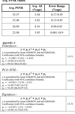
Next and given the VM values of “different” FR im-age face datasets, the effectiveness of this FR system performance prediction approach is of course of interest. Now and since in real life FR applications some type of compression coding may be used prior to FR, experiments were conducted with the previously employed 11 datasets being corrupted with coding noise introduced at different PSNR levels.

Furthermore the introduction of noise in input sample images can answer an important question i.e. how does the above derived FR system performance as related to VM models, which have been derived using noise-free image data, is affected by noisy input data? Or alterna-tively does the relationship defined between VM and system recognition performance also holds for noisy im-ages?

Thus experimentation was performed using JPEG coded face image datasets and according to the experi-mental set up of Fig. 8. This type of coding introduces a “block” type of noise/distortion. Note that for simplicity only the Fisherfaces FR approach was employed and

JPEG coding noise was adjusted at the four average PSNR values of 55.57, 33.48, 26.86, 23.98 dbs.

In Fig. 9 actual VM and recognition rate values are obtained using noisy input data at different PSNR values. Notice that a similar increasing trend in VM and recogni-tion performance values is observed in these curves, as in the case of noise free image based experimentation, see Fig. 5.

Moreover, curves are now shifted towards the bottom-left corner as the noise level increases. Thus a downward shift indicates that coding noise is suppressing facial vari-ation across different subjects, which in turn causes a decrease in recognition performance whereas a left shift shows that a simultaneous decrease in VM has

In addition, models derived from clean/un-coded data were employed to predict the recognition performance of systems operating on JPEG coded image data. The histo-grams of absolute prediction error (%age) for all the da-tasets and also percentage values of Average Absolute Errors (Avg. AE) corresponding to each average PSNR level are shown in Fig. 10 and Table-5, respectively. It is obvious from these values that in spite of introducing moderate image quality coding degradation in the input face images, model error ranges are approximately the same with those derived from noise-free data. This is indicative of the relative robustness of the proposed FRSP/VM system performance relationship with respect to coding distortion.

4. CONCLUSION

This paper investigated the modeling of FR system per-formance in terms of the signal variability measure de-rived from input image datasets. Thus a new variability measure (VM) that characterizes overall image face data variability has been defined and used over a number of well-known image datasets. In addition, relationships between such VM values and the performance of four conventional FR systems have been determined and mod-eled using second order polynomials. Note that the pro-posed VM measure takes into account both inter and intra correlation image dataset characteristics.

Thus computer simulation results involving 11 publi-cally available face image datasets show FRSP/VM pre-diction errors of less than 10%, for all four FR systems, and Avg. AE values across FR systems in the range of

3.27% and 5.47%. An increase in the number of availa-ble image datasets should further improve modeling accu-racy. Note: free availability of public face images datasets and complexity involved in recognition process are two major factors in using only 11 face images datasets in modeling process.

8

values. Prediction errors (i.e. Avg. AE) corresponding to face image data coded at different PSNR values shown that these noise-free FRSP/VM models kept their predic-tion accuracy to approximately the same level with that produced by noise-free input data. Moreover FRSP/VM curves show the same increasing trend as those of noise-free data. This suggests that any deterioration in recogni-tion performance, due to input image noise, is counterbal-anced by VM reductions so that the general FRSP/VM relationship is maintained.

REFERENCES

[1] Patel, Riddhi, and Shruti B. Yagnik. "A Literature Survey on Face Recognition Techniques." Interna-tional Journal of Computer Trends and Technology (IJCTT) 5.4 (2013): 189-194.

[2] Zhao, Wenyi, and Rama Chellappa. eds.

“

Face Pro-cessing: Advanced Modeling and Methods: Ad-vanced Modeling and Methods.” Academic Press,

2011.

[3] Li, Z. Stan, and Anil K. Jain. “Handbook of face recognition.” 2nd Editionspringer, 2011.

[4] Chellappa, Rama, Charles L. Wilson, and Saad Siro-hey. "Human and machine recognition of faces: A survey." Proceedings of the IEEE 83.5 (1995): 705-741.

[5] Lu, Yongzhong, Jingli Zhou, and Shengsheng Yu. "A survey of face detection, extraction and recogni-tion." Computing and informatics 22.2 (2003): 163-195.

[6] Tolba, A. S., A. H. El-Baz, and A. A. El-Harby. "Face Recognition: A Literature Re-view." International Journal of Signal Pro-cessing 2.2 (2006).

[7] Meethongjan, Kittikhun, and Dzulkifli Mohamad. "A Summary of literature review: Face Recogni-tion." (2007).

[8] Jafri, Rabia, and Hamid R. Arabnia. "A Survey of Face Recognition Techniques." JIPS 5.2 (2009): 41-68.

[9] Abate, Andrea F., et al. "2D and 3D face recogni-tion: A survey." Pattern Recognition Letters 28.14 (2007): 1885-1906.

[10]AT&T face database, AT&T Laboratories, Cambridge,

U.K, [Online] Available:

http://www.cl.cam.ac.uk/research/dtg/attarchive/facedataba se.html

[11] M.M. Nordstrøm, M. Larsen, J. Sierakowski, and M.B. Stegmann, “The imm face database-an annotated dataset of 240 face images,” Informatics and Mathematical Mod-eling, 2004.

[12]A. Georghiades, D. Kriegman, and P. Belhumeur, “From Few to Many: Generative Models for Recognition under Variable Pose and Illumination,” IEEE Trans. Pattern Analysis and Machine Intelligence, vol. 40, pp. 643-660, 2001.

[13]Georgia Tech Face Database, ftp://ftp.ee.gatech.edu/pub/users/hayes/facedb/.

[14]Stirling face database, [Online] Available: http://pics.stir.ac.uk

[15]Vidit Jain, Amitabha Mukherjee. The Indian Face Data-base.

http://vis-www.cs.umass.edu/~vidit/IndianFaceDatabase/ , 2002.

[16]FEI Face Database,

http://fei.edu.br/~cet/facedatabase.html.

[17]K Messer, J Matas, J Kittler, J Luettin, and G maitre. Xm2vtsdb: The extended m2vts database. In Second International Conference of Audio and Video-based Biometric Person Authentication, March 1999

[18]Daniel B Graham and Nigel M Allinson, “Character-izing Virtual Eigen signatures for General Purpose Face Recognition,” Face Recognition: From Theory to Applications, NATO ASI Series F, Computer and Systems Sciences, Vol. 163. H. Wechsler, P. J. Phil-lips, V. Bruce, F. Fogelman-Soulie and T. S. Huang (eds), pp 446-456, 1998.

[19]Bern Univ. Face Database,

ftp://iamftp.unibe.ch/pub/Images/FaceImages/, 2002.

[20]R. Singh, M. Vatsa, A. Ross, A. Noore, A mosaicing scheme for pose-invariant face recognition, IEEE Trans. Syst., Man, Cybern. B, Cybern. 37 (5) (2007) 1212–1225

[21]D. Beymer, T. Poggio, Face recognition from one example view, in: Proceedings of the International Conference on Computer Vision, 1995, pp. 500–507.

[22]Shaokang Chen and Brian C. Lovell, “Illumination

and Expression Invariant Face Recognition with One Sample Image”, ICPR, pp.300-303, 17th Internation-al Conference on Pattern Recognition (ICPR’ 04) – Volume 1, 2004

[23] S.J.D. Prince, J. Warrell, J.H. Elder, F.M. Felisberti, Tied factor analysis for face recognition across large pose differences, IEEE Trans. Pattern Anal. Mach. Intell. 30 (6) (2008) 970–984.

[24] P.J. Phillips, H. Wechsler, J. Huang, P. Rauss, The FERET database and evaluation procedure for face recognition algorithms, Image Vision Comput. 16 (5) (1998) 295–306.

[25] T. Sim, S. Baker, and M. Bsat, “The CMU pose,

9

[26] X. Chai, S. Shan, X. Chen, and W. Gao, “Locally

Linear Regression for Pose-Invariant Face Recogni-tion,” IEEE Trans. Image Processing, vol. 16, pp. 1716-1725, 2007.

[27]T. Kanade and A. Yamada, “Multi-Subregion-Based

Probabilistic Approach toward Pose-Invariant Face Recognition,” Proc. IEEE Int’l Symp. Computational Intelligence in Robotics and Automation, pp. 954-959, 2003

[28]O. Aghazadeh and S. Carlsson. Properties of Datasets Predict the Performance of Classifiers, Proc. British Machine Vision Conference (BMVC), pp. 44.1-44.10, 2013.

[29]J. P. Lewis, "Fast normalized cross-correlation."Vision interface. Vol. 10. No. 1. 1995.

[30]K.C. Lee and J. Ho and D. Kriegman, Acquiring Linear Subspaces for Face Recognition under Varia-ble Lighting, IEEE Trans. Pattern Anal. Mach. Intel-ligence. 27 (5) (2005) 684–698

[31]M. Turk and A. Pentland, "Face recognition using eigenfaces," IEEE Conference on Computer Vision andPattern Recognition, CVPR, 1991.

[32]F. Zhong, "L1-norm-based (2D)^2PCA," Conference on Computer Science and Electrical Engineering, pp. 1293-1296, 2013.

[33]T. Shakunaga and K. Shigenari, "Decomposed eigen face for face recognition under various lighting con-ditions," Proceedings of the 2001 IEEE Conference on Computer Vision and Pattern Recognition, CVPR, 2001.

[34]P. Belhumeur, J. Hespanha and D. Kriegman, "Eig faces vs. fisherfaces: Recognition using class specific linear projection," IEEE Transactions on Pattern Analysis and Machine Intelligence, PAMI, pp. 711-720, 1997.

[35]P.N. Belhumeur, J.P. Hespanha, D.J. Kriegman, Ei-genfaces vs. Fisherface: recognition using class spe-cific linear projection, IEEE Trans. Pattern Anal. Mach. Intell. 19 (7) (1997) 711–720.

[36]N. Kwak, J. Oh, Feature extraction for one-class classification problems: enhancements to biased dis-criminant analysis, Pattern Recognition 42 (2009) 17–26.

[37]Z.Z. Liang, Y.F. Li, P.F. Shi, A note on two-dimensional linear discriminant analysis, Pattern Recognition Letters 29 (2008) 2122–2128.

[38]L. Rueda, M. Herrera, Linear dimensionality reduction by maximizing the Chernoff distance in the transformed space, Pattern Recognition 41 (2008) 3138–3152.

[39]Y. Yan, Y.J. Zhang, A novel class-dependence feature analysis method for face recognition, Pattern Recognition Letters 29 (2008) 1907–1914.

[40]C. Cortes and V. Vapnik, "Support-vector networks," Ma-chine learning, vol. 20, pp. 273-297, 1995.

[41]C.W. Hsu and C.J. Lin. A comparison of methods for mul-ticlass support vector machins. IEEE Transactions on Neu-ral Networks, 13(2), March 2002.

[42]Theil, H., Economic forecasts and policy. 1958.

10

(a)

(b)

Fig.1: Normalized Histogram; a) is based on 𝐂̂1NCC

values obtained from a dataset with 10 images per subject which correspond to relatively small change in pose along the 0ofrom to 180orange. b) is based on set 𝐂̂2NCC

values obtained from a dataset with only three images per person representing pose rotations 0o, 90oand 180o.

Fig.2: Four face datasets are shown on x-axis. DS1 con-tains 3 images per subject with a 90o pose variation between successive images, whereas DS4 has 10 images per subject and the least pose variation across images. i.e. approximately 22.5o.

Fig.3: Examples of manually cropped images and their corresponding original images.

Fig.4: Experimental framework for evaluating prediction error ranges.

0 0.2 0.4 0.6 0.8 1

0.005 0.01 0.015 0.02 0.025 0.03 0.035

Normalized Cross-Correlation

O

c

c

u

r

r

e

n

c

e

s

0 0.2 0.4 0.6 0.8 1

0 0.005 0.01 0.015 0.02 0.025 0.03 0.035 0.04 0.045

Normalized Cross-Correlation

O

c

c

u

r

r

e

n

c

e

s

DS1 DS2 DS3 DS4

0.006 0.007 0.008 0.009 0.01 0.011 0.012

Face Datasets

In

tr

a

-s

u

b

je

ct

V

a

ri

a

b

il

it

y

Variability

Measure (VM) Predictor

Face Recognition

System VM

Prediction Model

Predicted Recognition Rate

Actual Recognition Rate

+

-Input Face Dataset Input Face Dataset

11

Fig.5: Recognition Rate Vs VM values obtained from 11 datasets and for four different FR systems

5 6 7 8 9 10 11 12 13 14 15

x 10-4 40

50 60 70 80 90 100

VM

R

ec

ogn

it

on

R

at

e

(%age

)

12

(a) (b)

(c) (d)

Fig.6: 𝐑𝟐 and 𝐑̅̅̅̅ 𝟐 Vs degree of Polynomial; a) Fisherfaces, b) PCA+SVM, c) Eigenfaces, and d) NCC.

Fig.7: Recognition Rate Vs VM values for a)

Fisherfaces, b) PCA+SVM, c) Eigenfaces, and d) NCC. 2nd degree polynomial models shown as dotted lines.

1 2 3 4 5 6 7

0.7 0.75 0.8 0.85 0.9 0.95 1 G ood ne ss of F it

Degree of Polynomial Model R-squared Adjusted R-squared

1 2 3 4 5 6 7

0.7 0.75 0.8 0.85 0.9 0.95 1 G ood ne ss of F it

Degree of Polynomial Model R-squared Adjusted R-squared

0.4 0.6 0.8 1 1.2 1.4 1.6

x 10-3 60 65 70 75 80 85 90 95 100 VM R ec ogn iti on R ate (%age ) True Data

2-Degree Polynomial Model 0.4 0.6 0.8 1 1.2 1.4 1.6

x 10-3

60 65 70 75 80 85 90 95 100 VM R ec ogn iti on R ate (%age ) True Data

2-Degree Polynomial Model

1 2 3 4 5 6 7

0.55 0.6 0.65 0.7 0.75 0.8 0.85 0.9 0.95

Degree of Polynomial Model

G ood ne ss of F it R-squared Adjusted R-squared

1 2 3 4 5 6 7

0.5 0.55 0.6 0.65 0.7 0.75 0.8 0.85 0.9 0.95 G ood ne ss of F it

Degree of Polynomial Model R-squared Adjusted R-squared

0.4 0.6 0.8 1 1.2 1.4 1.6

x 10-3 45 50 55 60 65 70 75 80 85 90 95 VM R ec ogn iti on R ate (%age ) True Data

2-Degree Polynomial Model 0.4 0.6 0.8 1 1.2 1.4 1.6

x 10-3 40 50 60 70 80 90 100 VM R ec ogn iti on R ate (%age ) True Data

13

Fig.8: Experimental framework for evaluating proposed VM using noisy data.

Fig.9: FRSP/VM curves corresponding to Fisherfaces FR system: same overall increasing trend as seen in Fig.5 can also be noticed in case of noise with all PSNR values.

0.4 0.6 0.8 1 1.2 1.4 1.6

x 10-3 60

65 70 75 80 85 90 95 100

VM

R

e

c

ogn

it

ion

R

at

e

(

%age

)

Avg. PSNR=55.5745 Avg. PSNR=31.8768 Avg. PSNR=26.8596 Avg. PSNR=23.9796

0 2 4 6 8 10

0 0.5 1 1.5 2 2.5 3

Absolute Error (%age)

N

o: of D

atas

ets

0 2 4 6 8 10

0 0.5 1 1.5 2 2.5 3

Absolute Error (%age)

N

o: of D

atas

ets

0 1 2 3 4 5 6 7 8 9

0 0.2 0.4 0.6 0.8 1 1.2 1.4 1.6 1.8 2

Absolute Error (%age)

N

o: of D

atas

ets

Variability Measure

(VM)

Predictor

Face Recognition

System VM

Prediction Model

Predicted Recognition Rate

Actual Recognition Rate

+

-Input Face Dataset Input Face Dataset

14

Fig.10: Histograms of Absolute Errors calculated using i) datasets corrupted by JPEG noise at four different PSNR values: a)

55.57, b) 33.48, c) 26.86, and d) 23.98. and ii) FRSP/VM models derived from clean data.

0 2 4 6 8 10 12

0 0.5 1 1.5 2 2.5 3

Absolute Error (%age)

N

o: of D

atas

[image:16.612.48.564.86.265.2]

15

Table 1: Some of the widely used Face Datasets in Face Recognition Applications

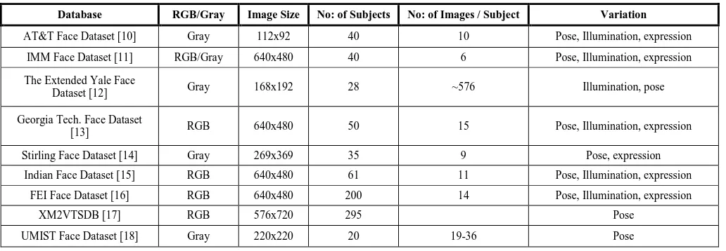
Database RGB/Gray Image Size No: of Subjects No: of Images / Subject Variation

AT&T Face Dataset [10] Gray 112x92 40 10 Pose, Illumination, expression

IMM Face Dataset [11] RGB/Gray 640x480 40 6 Pose, Illumination, expression

The Extended Yale Face

Dataset [12] Gray 168x192 28 ~576 Illumination, pose

Georgia Tech. Face Dataset

[13] RGB 640x480 50 15 Pose, Illumination, expression

Stirling Face Dataset [14] Gray 269x369 35 9 Pose, expression

Indian Face Dataset [15] RGB 640x480 61 11 Pose, Illumination, expression

FEI Face Dataset [16] RGB 640x480 200 14 Pose, Illumination, expression

XM2VTSDB [17] RGB 576x720 295 Pose

UMIST Face Dataset [18] Gray 220x220 20 19-36 Pose

Table 2: Face Datasets having Pose Variation

Database No: of Subjects Pose Variation

AT&T Face Dataset [10] 40 10 random poses within ±20 in Yaw and Tilt Bern Uni Face Dataset [19] 30 5 poses: 0o_{, ±20 in Yaw and Tilt}

XM2VTSDB [17] 125 5 poses: 0o_{, ±30 in Yaw and Tilt}

WVU [20] 40 7 poses: 0o_{, ±20, ±40, ±60 in Yaw}

[image:16.612.133.482.303.424.2]

[image:17.595.307.565.67.206.2]

16

Table 3: Recognition Rate reported for different Pose Variation

Database No: of

Subjects

Pose Difference among Images

Reported Recognition

Rate FERET

[24] 100 22.5

o _{/ 67.5}o _{/ 90}o _{100 / 99 / 92 [23]}

CMU PIE

[25] 68 16

o _{/ 45}o _{99.85 / 89.7 [26]}

CMU PIE

[25] 34 45

o _{/ 67.5}o _{/ 90}o _{100 / 80 / 40 [27]}

Table 4: Parameters for 2nd-degree Polynomial Model

FR Systems 𝑅2 𝑅̅̅̅̅2 Avg. AE (%age)

Error Range (%age)

Fisherfaces 0.827 0.783 3.27 0.13-8.5

PCA+SVM 0.837 0.796 3.63 0.41-8.7

Eigenfaces 0.889 0.860 4.40 1.08-8.1

[image:17.595.46.285.124.290.2]

NCC 0.8510 0.814 5.47 2.08-11.1

Table 5: Avg. Absolute Error (Avg. AE) at different Avg. PSNR values.

Avg. PSNR Avg. AE (%age)

Error Range (%age)

55.57 3.54 0.17-9.59

33.48 3.82 0.13-9.85

26.86 4.16 0.86-8.01

23.98 3.95 0.001-10.9

Appendix-A Fisherfaces:-

𝑦 = 𝑝1𝑥2+ 𝑝2𝑥 + 𝑝3

𝑥 is normalized by mean 0.000878 and std 0.0003201. Coefficients (with 95% confidence bounds).

𝑝1= −5.188 (−9.211, −1.165)

𝑝2= 10.38 (6.5,14.25)

𝑝3= 89.53 (84.6,94.46)

(A-1)

PCA+SVM:-𝑦 = 𝑝1𝑥2+ 𝑝2𝑥 + 𝑝3

𝑥 is normalized by mean 0.000878 and std 0.0003201. Coefficients (with 95% confidence bounds).

𝑝1= −6.926 (−11.54, −2.31)

𝑝2= 12.28 (7.827,16.72)

𝑝3= 91.69 (86.04,97.35)

(A-2)

Eigenfaces:-

𝑦 = 𝑝1𝑥2+ 𝑝2𝑥 + 𝑝3

𝑥 is normalized by mean 0.000878 and std 0.0003201. Coefficients (with 95% confidence bounds).

𝑝1= −6.919 (−11.9, −1.933)

𝑝2= 16.58 (11.78,21.39)

(A-3)

𝑝₃= 79.08 (72.97,85.18)

NCC:-

𝑦 = 𝑝1𝑥2+ 𝑝2𝑥 + 𝑝3

𝑥 is normalized by mean 0.000878 and std 0.0003201. Coefficients (with 95% confidence bounds).

𝑝1= −6.632 (−12.69, −0.5738)

𝑝2= 17.05 (11.21, 22.89)

𝑝3= 80.23 (72.81, 87.65)

(A-4)

[image:17.595.47.300.392.779.2]