Exploring Text and Image Features to Classify Images in Bioscience Literature

(1)

Exploring Text and Image Features to Classify Images in Bioscience

Lit-erature

Barry Rafkind Minsuk Lee Shih-Fu Chang Hong Yu

DVMM Group Department of Health Sci-ences

Columbia University University of Wisconsin-Milwaukee

Columbia University University of Wisconsin-Milwaukee New York, NY 10027 Milwaukee, WI 53201 New York, NY 10027 Milwaukee, WI 53201 Barryr

@ee.columbia.edu

Minsuk.Lee @gmail.com

Sfchang @ee.columbia.edu

Hong.Yu @uwm.edu

Abstract

A picture is worth a thousand words. Biomedical researchers tend to incorpo-rate a significant number of images (i.e., figures or tables) in their publications to report experimental results, to present re-search models, and to display examples of biomedical objects. Unfortunately, this wealth of information remains virtually inaccessible without automatic systems to organize these images. We explored su-pervised machine-learning systems using Support Vector Machines to automatically classify images into six representative categories based on text, image, and the fusion of both. Our experiments show a significant improvement in the average F-score of the fusion classifier (73.66%) as compared with classifiers just based on image (50.74%) or text features (68.54%).

1 Introduction

A picture is worth a thousand words. Biomedical researchers tend to incorporate a significant num-ber of figures and tables in their publications to report experimental results, to present research models, and to display examples of biomedical objects (e.g., cell, tissue, organ and other images). For example, we have found an average of 5.2 im-ages per biological article in the journal Proceed-ings of the National Academy of Sciences (PNAS). We discovered that 43% of the articles in the

medical journal The Lancet contain biomedical images. Physicians may want to access biomedical images reported in literature for the purpose of clinical education or to assist clinical diagnoses. For example, a physician may want to obtain im-ages that illustrate the disease stage of infants with Retinopathy of Prematurity for the purpose of clinical diagnosis, or to request a picture of ery-thema chronicum migrans, a spreading annular rash that appears at the site of tick-bite in Lyme disease. Biologists may want to identify the ex-perimental results or images that support specific biological phenomenon. For example, Figure 1 shows that a transplanted progeny of a single mul-tipotent stem cell can generate sebaceous glands.

Organizing bioscience images is not a new task. Related work includes the building of domain-specific image databases. For example, the Protein Data Bank (PDB) 1 (Sussman et al., 1998) stores 3-D images of macromolecular structure data. WebPath 2 is a medical web-based resource that has been created by physicians to include over 4,700 gross and microscopic medical images. Text-based image search systems like Google ignore image content. The SLIF (Subcellular Location Image Finder) system (Murphy et al., 2001; Kou et al., 2003) searches protein images reported in lit-erature. Other work has explored joint text-image features in classifying protein subcellular location images (Murphy et al., 2004). The existing sys-tems, however, have not explored approaches that automatically classify general bioscience images into generic categories.

1

http://www.rcsb.org/pdb/

2

http://www-medlib.med.utah.edu/WebPath/webpath.html

(2)

Classifying images into generic categories is an important task that can benefit many other natural language processing and image processing tasks. For example, image retrieval and question answer-ing systems may return “Image-of-Thanswer-ing” images (e.g., Figure 1), not the other types (e.g., Figure 2~5), to illustrate erythema chronicum migrans. Biologists may examine “Gel” images (e.g., Figure 2), rather than “Model” (e.g., Figure 4) to access specific biological evidence for molecular interac-tions. Furthermore, a generic category may ease the task of identifying specific images that may be sub-categories of the generic category. For exam-ple, a biologist may want to obtain an image of a protein structure prediction, which might be a sub-category of “Model” (Figure 4), rather than an im-age of x-ray crystallography that can be readily obtained from the PDB database.

This paper represents the first study that defines a generic bioscience image taxonomy, and ex-plores automatic image classification based on the fusion of text and image classifiers.

Gel-Image consists of gel images such as Northern

(for DNA), Southern (for RNA), and Western (for protein). Figure 2 shows an example.

Graph consists of bar charts, column charts, line

charts, plots and other graphs that are drawn either by authors or by a computer (e.g., results of patch clamping). Figure 3 shows an example.

Image-of-Thing refers to images of cells, cell

components, tissues, organs, or species. Figure 1 shows an example.

Mix refers to an image (e.g., Figure 5) that

incor-porates two or more other categories of images.

Model: A model may demonstrate a biological

process, molecular docking, or an experimental design. We include as Model any structure (e.g., chemical, molecular, or cellular) that is illustrated by a drawing. We also include gene or protein se-quences and sequence alignments, as well as phy-logenetic trees in this category. Figure 4 shows one example.

Table refers to a set of data arranged in rows and

columns.

Table 1. Bioscience Image Taxonomy

2 Image Taxonomy

We downloaded from PubMed Central a total of 17,000 PNAS full-text articles (years 1995-2004), which contain a total of 88,225 images. We manu-ally examined the images and defined an image taxonomy (as shown in Table 1) based on feedback from physicians. The categories were chosen to maintain balance between coherence of content in each category and the complexity of the taxonomy. For example, we keep images of biological objects (e.g., cells, tissues, organs etc) in one single cate-gory in this experiment to avoid over decomposi-tion of categories and insufficient data in individual categories. Therefore we stress princi-pled approaches for feature extraction and classi-fier design. The same fusion classification framework can be applied to cases where each category is further refined to include subclasses.

Figure 1. Image of_Thing3

Figure 2. Gel image4

Figure 3. Graph image5_{Figure 4. Model image}6

Figure 5. Mix image7

3

This image appears in the cover page of PNAS 102 (41): 14477 – 14936.

4

The image appears in the article (pmid=10318918)

5

6

7

(3)

3 Image Classification

We explored supervised machine-learning methods to automatically classify images according to our image taxonomy (Table 1). Since it is straightfor-ward to distinguish table separately by applying surface cues (e.g., “Table” and “Figure”), we have decided to exclude it from our experiments.

3.1 Support Vector Machines

We explored supervised machine-learning systems using Support Vector Machines (SVMs) which have shown to out-perform many other supervised machine-learning systems for text categorization tasks (Joachims, 1998). We applied the freely available machine learning MATLAB package The

Spider to train our SVM systems (Sable and

Wes-ton, 2005; MATLAB). The Spider implements many learning algorithms including a multi-class SVM classifier which was used to learn our dis-criminative classifiers as described below in sec-tion 3.4.

A fundamental concept in SVM theory is the projection of the original data into a high-dimensional space in which separating hyperplanes can be found. Rather than actually doing this pro-jection, kernel functions are selected that effi-ciently compute the inner products between data in the high-dimensional space. Slack variables are introduced to handle non-separable cases and this requires an upper bound variable, C.

Our experiments considered three popular ker-nel function families over five different variants and five different values of C. The kernel function implementations are explained in the software documentation. We considered kernel functions in the forms of polynomial, radial basis function, and Gaussian. The adjustable parameter for polynomial functions is the order of the polynomial. For radial basis function and Gaussian functions, sigma is the adjustable parameter. A grid search was performed over the adjustable parameter for values 1 to 5 and for values of C equal to [10^0, 10^1, 10^2, 10^3, 10^4].

3.2 Text Features

Previous work in the context of newswire image classification show that text features in image cap-tions are efficient for image categorization (Sable, 2000, 2002, 2003). We hypothesize that image

captions provide certain lexical cues that effi-ciently represent image content. For example, the words “diameter”, “gene-expression”, “histogram”, “lane”, “model“, “stained”, “western”, etc are strong indicators for image classes and therefore can be used to classify an image into categories. The features we explored are bag-of-words and n-grams from the image captions after processing the caption text by the Word Vector Tool (Wurst).

3.3 Image Features

We also investigated image features for the tasks of image classification. We started with four types of image features that include intensity histogram features, direction histogram features, edge-based axis features, and the number of 8-connected regions in the binary-valued image obtained from thresholding the intensity.

The intensity histogram was created by quantiz-ing the gray-scale intensity values into the range 0-255 and then making a 256-bin histogram for these values. The histogram was then normalized by di-viding all values by the total sum. For the purpose of entropy calculations, all zero values in the his-togram are set to one. From this adjusted, normal-ized histogram, we calculated the total entropy as the sum of the products of the entries with their logarithms. Additionally, the mean, 2nd moment, and 3rd moment are derived. The combination of the total entropy, mean, 2nd, and 3rd moments constitute a robust and concise representation of the image intensity.

(4)

entropy, mean, 2nd and 3rd moments are extracted to summarize the EDH.

The edge-based axis features are meant to help identify images containing graphs or charts. First, Sobel edges are extracted above a sensitivity threshold of 0.10 from the gray-scale image. This yields a binary-valued intensity image with 1’s occurring in locations of all edges that exceed the threshold and 0’s occurring otherwise. Next, the vertical and horizontal sums of this intensity image are taken yielding two vectors, one for each axis. Zero values are set to one to anticipate the entropy calculations. Each vector is then normalized by dividing each element by its total sum. Finally, we find the total entropy, mean, 2nd , and 3rd mo-ments to represent each axis for a total of eight axis features.

The last image feature under consideration was the number of 8-connected regions in the binary-valued, thresholded Sobel edge image as described above for the axis features. An 8-connected region is a group of edge pixels for which each member touches another member vertically, horizontally, or diagonally in the eight adjacent pixel positions sur-rounding it. The justification for this feature is that the number of solid regions in an image may help separate classes.

A preliminary comparison of various combina-tions of these image features showed that the inten-sity histogram features used alone yielded the best classification accuracy of approximately 54% with a quadratic kernel SVM using an upper slack limit of C = 10^4.

3.4 Fusion

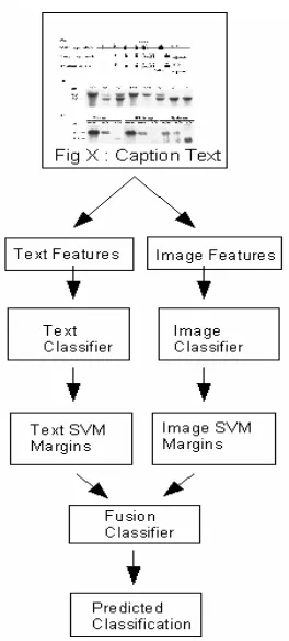
We integrated both image and text features for the purpose of image classification. Multi-class SVM’s were trained separately on the image features and the text features. A multi-class SVM attempts to learn the boundaries of maximal margin in feature space that distinguishes each class from the rest. Once the optimal image and text classifiers were found, they were used to process a separate set of images in the fusion set. We extracted the margins from each data point to the boundary in feature space.

Thus, for a five-class classifier, each data point would have five associated margins. To make a fair comparison between the image-based classifier and the text-based classifier, the margins for each

data point were normalized to have unit magnitude. So, the set of five margins for the image classifier constitutes a vector that then gets normalized by dividing each element by its L2 norm. The same is done for the vector of margins taken from the text classifier. Finally, both normalized vectors are concatenated to form a 10-dimensional fusion vec-tor. To fuse the margin results from both classifi-ers, these normalized margins were used to train another multi-class SVM.

A grid search through parameter space with cross validation identified near-optimal parameter settings for the SVM classifiers. See Figure 6 for our system flowchart.

Figure 6. System Flow-chart

3.5 Training, Fusion, and Testing Data

We randomly selected a subset of 554 figure im-ages from the total downloaded image pool. One author of this paper is a biologist who annotated figures under five classes; namely, Gel_Image (102), Graph (179), Image_of_Thing (64), Mix (106), and Model (103).

(5)

classi-fiers for the image-based and text-based features. The fusion set was used to train a classifier on top of the results of the image-based and text-based classifiers. The testing set was used to evaluate the final classification system.

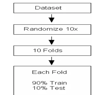
For each division of data, 10 folds were gener-ated. Thus within the training and fusion data sets, there are 10 folds which each have a randomized partitioning into 90% for training and 10% for test-ing. The testing data set did not need to be parti-tioned into folds since all of it was used to test the final classification system. (See Figure 8).

In the 10-fold cross-validation process, a classi-fier is trained on the training partition and then measured for accuracy (or error rate) on the testing partition. Of the 10 resulting algorithms, the one which performs the best is chosen (or just one which ties for the best accuracy).

Figure 7. Image-set Divisions

3.6 Evaluation Metrics

We report the widely used recall, precision, and F-score (also known as F-measure) as the evaluation metrics for image classification. Recall is the total number of true positive predictions divided by the total number of true positives in the set (true pos + false neg). Precision is the fraction of the number of true positive predictions divided by the total number of positive predictions (true pos + false pos). F-score is the harmonic mean of recall and precision equal to (C. J. van Rijsbergen, 1979):

(

precision recall

)

recall

precision* / +

* 2

Figure 8. Partitioning Method for Training and

Fusion Datasets

4 Experimental Results

Table 2 shows the Confusion Matrix for the image feature classifier obtained from the testing part of the training data. The actual categories are listed vertically and predicted categories are listed hori-zontally. For instance, of 26 actual GEL images, 18 were correctly classified as GEL, 4 were mis-classified as GRAPH, 2 as IMAGE_OF_THING, 0 as MIX, and 2 as MODEL.

Actual Predicted Categories

Gel Graph Thing Mix Model

Gel 18 4 2 0 2

Graph 3 39 0 1 1

Img_Thing 1 1 12 2 0

Mix 4 17 0 3 3

Model 8 13 0 1 3

Table 2. Confusion Matrix for Image Feature

Clas-sifier

(6)

were classified as the most popular category, GRAPH. Clearly, the image-based classifier does best at recognizing IMAGE_OF_THING figures.

Category TP FP FN Prec. Recall Fscore Gel 18 16 8 0.529 0.692 0.600 Graph 39 35 5 0.527 0.886 0.661 Img_Thing 12 2 4 0.857 0.750 0.800 Mix 3 4 10 0.429 0.231 0.300 Model 3 6 22 0.333 0.120 0.176 Table 3. Precision, Recall, F-score for Image

Clas-sifier

Gel 22 2 0 2 0

Graph 4 36 0 4 0

Mix 3 9 1 12 2

Model 3 5 0 3 14

Table 4. Confusion Matrix for Caption Text

Clas-sifier

Category TP FP FN Prec Recall Fscore Gel 22 10 4 0.688 0.845 0.758 Graph 36 19 8 0.655 0.818 0.727 Img_Thing 11 1 5 0.917 0.688 0.786 Mix 12 10 15 0.545 0.444 0.489 Model 14 3 11 0.824 0.560 0.667 Table 5. Precision, Recall, F-score for Caption

Text Classifier

The text-based classifier excels in finding GEL, GRAPH, and IMAGE_OF_THING images. It achieves an accuracy of (22+36+11+12+14)/138 = 95/138 = 69%.

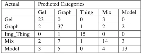
A near-optimal parameter setting for the fusion classifier based on both image features and text features used a linear kernel with C = 10. The cor-responding Confusion matrix follows in Table 6.

Gel 23 0 0 3 0

Graph 2 37 1 2 2

Mix 2 7 1 14 3

Model 3 5 0 4 13

Table 6. Confusion Matrix for Fusion Classifier

Category TP FP FN Prec. Recall Fscore Gel 23 7 3 0.767 0.885 0.822 Graph 37 13 7 0.740 0.841 0.787 Img_Thing 15 2 1 0.882 0.938 0.909 Mix 14 9 13 0.609 0.519 0.560 Model 13 5 12 0.722 0.520 0.605 Table 7. Precision, Recall, F-score for Fusion

Classifier

From Table 7, it is apparent that the fusion clas-sifier does best on IMAGE_OF_THING and also performs well on GEL and GRAPH. These are substantial improvements over the classifiers that were based on image or text feature alone. Average F-scores and accuracies are summarized below in Table 8.

The overall accuracy for the fusion classifier = sum of true positives / total number of image = (23+37+15+14+13)/138 = 102/138 = 74%. This can be compared with the baseline of 44/138 = 32% if all images were classified as the most popu-lar category, GRAPH.

Classifier Average F-score Accuracy Image 50.74% 54% Caption

Text

68.54% 69%

Fusion 73.66% 74%

Table 8. Comparison of Average F-scores and

Ac-curacy among all three Classifiers

5 Discussion

It is not surprising that the most difficult category to classify is Mix. This was due to the fact that Mix images incorporate multiple categories of other image types. Frequently, one other image type that appears in a Mix image dominates the image fea-tures and leads to its misclassification as the other image type. For example, Figure 9 shows that a Mix image was misclassified as Gel_Image.

This mistake is forgivable because the image does contain sub-images of gel-images, even though the entire figure is actually a mix of gel-images and diagrams. This type of result highlights the overlap between classifications and the diffi-culty in defining exclusive categories.

(7)

intuitive understanding of discriminative behavior of SVM classifiers is a valid criticism of the tech-nique. Although generative machine learning methods (such as Bayesian techniques or Graphical Models) offer more intuitive models for explaining success or failure, discriminative models like SVM are adopted here due to their higher performance and ease of use.

Figure 10 shows an example of a MIX figure that was mislabeled by the image classifier as GRAPH and as GEL_IMAGE by the text classi-fier. However, it was correctly labeled by the fu-sion classifier. This example illustrates the value of the fusion classifier for being able to improve upon its component classifiers.

6 Conclusions

From the comparisons in Table 8, we see that fus-ing the results of classifiers based on text and im-age features yields approximately 5% improvement over the text -based classifier alone with respect to both average F-score and Accuracy. In fact, the F-score improved for all categories ex-cept for MODEL which experienced a 6% drop. The natural conclusion is that the fusion classifier combines the classification performance from the text and image classifiers in a complementary fash-ion that unites the strengths of both.

7 Future Work

To enhance the performance of the text features, one may restrict the vocabulary to functionally im-portant biological words. For example, “phos-phorylation” and “3-D” are important words that might sufficiently separate “protein function” from “protein structure”.

Further experimentation on a larger image set would give us even greater confidence in our re-sults. It would also expand the diversity within each category, which would hopefully lead to bet-ter generalization performance of our classifiers.

Other possible extensions of this work include investigating different machine learning ap-proaches besides SVMs and other fusion methods. Additionally, different sets of image and text fea-tures can be explored as well as other taxonomies.

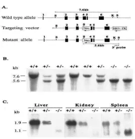
Caption: ”The 2.6-kb HincII XhoI fragment con-taining approximately half of exon 4 and exon 5 and 6 was subcloned between the Neo gene and thymidine kinase (Fig. 1 A). The location of the genomic probe used to screen for homologous re-combination is shown in Fig. 1 A. Gene Targeting in Embryonic Stem (ES) Cells and Generation of Mutant Mice. Genomic DNA of resistant clones was digested with SacI and hybridized with the 3 0.9-kb KpnI SacI external probe (Fig. 1 A). Chi-meric male offspring were bred to C57BL/6J fe-males and the agouti F1 offspring were tested for transmission of the disrupted allele by Southern blot analysis of SacI-digested genomic DNA by using the 3 external probe (Fig. 1 A and B). A 360-bp region, including the first 134 360-bp of the 275-360-bp exon 4, was deleted and replaced with the PGKneo cassette in the reverse orientation (Fig. 1 A). After selection with G418 and gangciclovir, doubly sistant clones were screened for homologous re-combination by Southern blotting and hybridization with a 3 external probe (Fig. 1 A). Offspring were genotyped by Southern blotting of genomic tail DNA and hybridized with a 3 external probe (Fig. 1 B). To confirm that HFE / mice do not express the HFE gene product, we performed Northern blot analyses “

Figure 9. Above, caption text and image of a MIX

(8)

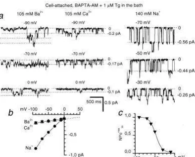
“Conductance properties of store-operated channels in A431 cells. (a) Store-operated channels in A431 cells, activated by the mixture of 100 mM BAPTA-AM and 1 mM Tg in the bath solution, were recorded in c/a mode with 105 mM Ba2+ (Left), 105 mM Ca2+ (Center), and 140 mM Na+ (Right) in the pipette solution at mem-brane potential as indicated. (b) Fit to the unitary cur-rent-voltage relationship of store-operated channels with Ba2+ (n = 46), Ca2+ (n = 4), Na+ (n = 3) yielded slope single-channel conductance of 1 pS for Ca2+ and Ba2+ and 6 pS for Na+. (c) Open channel probability of store-operated channels (NPomax30) expressed as a function of membrane potential. Data from six independent ex-periments in c/a mode with 105 mM Ba2+ as a current carrier were averaged at each membrane potential. (b and c) The average values are shown as mean ± SEM, unless the size of the error bars is smaller than the size of the symbols.”

Figure 10. Above, caption text and image of a

MIX figure incorrectly labeled as GRAPH by Im-age Classifier and GEL_IMAGE by the Text Clas-sifier

Acknowledgements

We thank three anonymous reviewers for their valuable comments. Hong Yu and Minsuk Lee ac-knowledge the support of JDRF 6-2005-835.

References

Anil K. Jain and A. Vailaya., August 1996, Image re-trieval using color and shape. Pattern Recognition, 29:1233–1244

Anil K. Jain, Fundamentals of Digital Image Processing, Prentice Hall, 1989

C. J. van Rijsbergen. Information Retrieval. Butter-worths, London, second edition, 1979.

Joachims T, 1998, Text categorization with support vec-tor machines: Learning with many relevant features.

Presented at Proceedings of ECML-98, 10th Euro-pean Conference on Machine Learning

Kou, Z., W.W. Cohen and R.F. Murphy. 2003. Extract-ing Information from Text and Images for Location Protemics, pp. 2-9. In ACM SIGKDD Workshop on Data Mining in Bioinformatics (BIOKDD).

Murphy, R.F., M. Velliste, J. Yao, and P.G. 2001. Searching Online Journals for Fluorescence Micro-scope Images depicting Protein Subcellular Location Patterns, pp. 119-128. In IEEE International Sympo-sium on Bio-Informatics and Biomedical Engineering (BIBE).

Murphy, R.F., Kou, Z., Hua, J., Joffe, M., and Cohen, W. 2004. Extracting and structuring subcellular lo-cation information from on-line journal articles: the subcellular location image finder. In Proceedings of the IASTED International Conference on Knowledge Sharing and Collaborative Engineering (KSCE2004), St. Thomas, US Virgin Islands, pp. 109-114.

Sable, C. and V. Hatzivassiloglou. 2000. Text-based approaches for non-tropical image categorization. International Journal on Digital Libraries. 3:261-275.

Sable, C., K. McKeown and K. Church. 2002. NLP found helpful (at least for one text categorization task). In Proceedings of Empirical Methods in Natu-ral Language Processing (EMNLP). Philadelphia, PA

Sable, C. 2003. Robust Statistical Techniques for the Categorization of Images Using Associated Text. In Computer Science. Columbia University, New York.

Sussman J.L., Lin D., Jiang J., Manning N.O., Prilusky J., Ritter O., Abola E.E. (1998) Protein Data Bank (PDB): Database of Three-Dimensional Structural In-formation of Biological Macromolecules. Acta Crys-tallogr D Biol CrysCrys-tallogr 54:1078-1084

MATLAB ™. The Mathworks Inc., http://www.mathworks.com/

Weston, J., A. Elisseeff, G. BakIr, F. Sinz. Jan. 26th, 2005. The SPIDER: object-orientated machine learn-ing library. Version 6. MATLAB Package. http://www.kyb.tuebingen.mpg.de/bs/people/spider/

Wurst, M., Word Vector Tool, Univeristät Dortmund,