Behind the Times
: Detecting Epoch Changes using Large Corpora
Octavian Popescu and Carlo Strapparava
FBK-irst, Trento, Italy
{popescu,strappa}@fbk.eu
Abstract
Using large corpora of chronologically or-dered language, it is possible to explore diachronic phenomena, identifying previ-ously unknown correlations between lan-guage usage and time periods, or epochs. We focused on a statistical approach to epoch delimitation and introduced the task of epoch characterization. We investi-gated the significant changes in the distri-bution of terms in the Google N-gram cor-pus and their relationships with emotion words. The results show that the method is reliable and the task is feasible.
1 Introduction
Traditionally, scholars of history define epochs ac-cording to their deep knowledge and understand-ing of facts over a long stretch of time. Intuitively, in order to define a new epoch, both a big social impact of a series of events and new issues, which arouse the social interest, must be observed. How-ever, it is hard to define what makes a feature “dis-tinctive” or an event a “great change”. It is even harder to evaluate and measure the impact of a series of changes in society in an objective way. Since the advent of regular newspapers and the in-dustry of mass media, written information has rep-resented a mirror of the interests of society. A so-cial event is relevant only if people pay attention to it and comment on it. A major change in so-ciety is reflected in the frequencies with which a set of topics is mentioned in mass media, some of them becoming mentioned more often than previ-ously, while some others are no more of interest. Furthermore, specific epochs typically develop a particular form of wording or rhetorical style.
In this paper we describe a computational ap-proach toepoch delimitationon the basis of word distribution over certain periods of time. A big
quantity of data, chronologically ordered, allows accurate statistical statements regarding the co-variance between the frequencies of two or more terms over a certain period of time. By discov-ering significant statistical changes in word usage behavior, it is possible to define epoch boundaries. We show that it is possible to distinguish a se-ries of limited periods of time, spanning at most three years, within which non-random changes af-fect the joint distribution of terms. Between two such short periods (i.e. the boundaries) no statis-tical significant changes are observed for decades, and thus we can refer to it as an epoch. The dis-tributions of the considered terms before and after boundaries are distinctly different.
We also introduce the task ofepoch
character-ization. Certain words carry with them an
emo-tional charge, like joy, fear, disgust etc. Within a given epoch, we can analyze the distribution of emotion words and their co-occurrences with the set of terms considered indicative for epoch def-inition. The pattern of these co-occurrences con-stitutes a blueprint of emotional tendencies with respect to some particular topics in the society within a certain period. Given an arbitrary sam-ple of data from a given, but unknown period of time, the task consists in correlating the emotional pattern of the data with the one of an epoch from which the data comes. The experiments reported here show that this task is feasible and sensible re-sults are obtained.
The corpus used in the current experiments is the Google 5-grams made of all tuples of consec-utive 5 words, coming from English books printed roughly from 1614 to 2009.
For the purpose of the present paper, we com-piled a lexicon of political and social terms. The lexicon contains 761 words, such as: capitalism,
civil disobedience,demagogue,democracy,
dicta-tor, chickenhawk, education, government, peace,
war etc. The these terms come from the lists
compiled for the political and sociological domain publicly available1. The frequency of these terms and their covariance is analyzed over the years and non-random changes are found according to the methodology presented in Section 3. The method-ology itself is purely statistical and it does not de-pend in any way on what the list contains. We could have equally chosen terms from art or sport domain, obtaining epoch boundaries specific to each domain.
The emotion words used in epoch characteriza-tion come primarily from the NRC Word-Emocharacteriza-tion Association Lexicon (Mohammad and Turney, 2010) to which the list of emotion words extracted from WordNet-Affect (Strapparava and Valitutti, 2004), distributed in the Semeval 2007 Affective Text task (Strapparava and Mihalcea, 2007), has been added. The lexicon is made up of English words to which eight possible tags are attached:
anger, anticipation, disgust, fear, joy, sadness,
surprise and trust. All in all there are 14,000
words for which at least one affective tag is given. The paper is organized as follows. In Sec-tion 2 we review the relevant literature. Sec-tion 3 presents the statistical apparatus employed in epoch determination and epoch characteriza-tion. In Section 4 we present the experiments and the results we have obtained. In the last section we highlight the contribution of this paper and make an overview of further immediate work.
2 Related Work
In (Michel et al., 2011), besides a complete intro-duction to the Google Books corpus, a limited di-achronic study of words meaning and form is also carried out. The authors introduce the term ‘cul-turomic’ and show that quantitative analyses may lead to interesting results. They show that it is possible to determine censorship and suppression by comparing the frequencies of proper names in bilingual Google books corpora. However, the au-thors did not proceed to a systematic studies of epochs.
Regarding semantic change, the task of sense disambiguation over the years is introduced in (Mihalcea and Nastase, 2012). In their paper, the authors refer to definite periods of time as epochs but they considered them prior defined.
In (Wang and Mccallum, 2006) an analysis of topics over time is carried out. The paper
fo-1E.g.www.democracy.org.au/glossary.html
cuses on rather fixed topics, which are expressed by frozen compounds, such as “mexican war”, “CVS operation”, and determines how these top-ics evolve during the years. However, because the scope of their paper is not global, the corpus used comes from 19 months of personal emails. It is hard to see how this method could general-ize. A similar approach is described in (Wang et al., 2008). The authors use LDA to facilitate the search into large corpora by automatically orga-nizing them.
In (Yu et al., 2010), the statistics tests and the google N-gram corpus are used for (semi) auto-matic creation and validation of a sense pool. The frequencies extracted from Google N-gram corpus are filtered with an appropriate statistical test and further verified by human experts.
The richness and complexity of cultural infor-mation contained in the Google N-gram corpus is analyzed in (Joula, 2012). By considering the degree of interdependence as a measure for com-plexity, the author used the 2-gram corpus to an-alyze the complexity of American culture. How-ever, there is no the epoch distinction and statisti-cal support.
Regarding Sentiment analysis, text categoriza-tion according to affective relevance, opinion ex-ploration for market analysis, etc. are just some examples of application this NLP area (Pang and Lee, 2008). While positive/negative valence checking is an active field of sentiment analysis, a fine-grained emotion checking is nowadays an emerging research topic. For example, SemEval task on Affective Text (Strapparava and Mihalcea, 2007) focussed on the recognition of six emotions emotions in a corpus of news headlines.
3 Methodology
5-gram corpus:
n-grams year # occ. # pages # books
democracy at work 1996 1 1 1
democracy at work 1997 5 5 5
democracy at work 1998 2 2 2
Table 1: 5-Gram Google files
3.1 Statistical tests
Normalization. Due to the exponential growth
of the published data, it is better to normalize the number of occurrences for a meaningful compari-son. We considered all the content nouns, includ-ing proper names, and we computed for each term of interest the percentage of occurrences of that term with respect to the sum of frequencies of all content nouns (considering lemmata). In this pa-per, when we refer to frequency of a term we mean the normalized figure, unless explicitly stated oth-erwise. The percentage is in fact very informative on what the public opinion is concerned about in certain periods and substantial differences may be observed within a short period of time. For
exam-ple,democracywas 25 times less a probable topic
at the begin of twenty-first century than 50 years before. In such cases, one can clearly talk about a change of interest in society, see Figure 1.
Welch’s test. Welch test is a variant of t-student
test to check whether two different samples come from the same population or not (Sawilowsky, 2001). The Welch test fits our purposes because it does not assume that the sample have equal vari-ance, thus it can be applied where the other similar tests, such as classical t-student or F-test, do not. The initial conditions for Welch test does not in-clude (1) the equality of the sample sizes and (2) either the homogeneity of population, thus the data may not come from a population having a distribu-tion with a unique variance. In fact for this reason we prefer to use non parametric test in the present paper.
In practice, we apply the Welch’s test to sample size representing contiguous periods of time . To exemplify, let us consider here the term “war” and two different periods 1800-1900 and 1900-2000. Each period is split in two sub-periods, 1800-1850 vs. 1850-1900, and 1900-1950 vs. 1950-2000 re-spectively. We test whether the samples 1800-1850 vs. 1800-1850-1900 have the same mean, and we also test whether the samples 1900-1950 vs.
1950-2000 have the same mean. In Table 2 we present the results obtained.
Sample t Outcome
1800-1850 vs. 1850-1900
µ1= .078 vs.µ2=.081 0.23 No Rejection atα= 0.1
1900-1950 vs. 1950-2000
µ1= .184 vs.µ2=.098 -5.163 Rejection atα= 0.01
Table 2: Welch’s test for termwar.
The null hypothesis, that the two sample come from a population with the same mean cannot be rejected atα= 0.1in the first case. The same null hypothesis is rejected with a very high confidence,
α= 0.01in the second case.
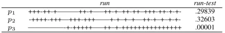
Run Test. Run test is a non parametric test,
which determines whether the a sequence of num-bers is likely to be the result of a random process or there might be an inner pattern in data (Gibbons and Chakraborti, 1992; Lindgren, 1993). For ex-ample let us suppose that we have a Bernoulli pro-cess with “+” and “-” possible outcomes and prob-abilities 1/4, 3/4 respectively. A sequences like ++++———-+++++——— is very unlikely to be a random generated sequences of this process. The run test is designed to detect such cases. A set of real values, as the frequencies of a term over a pe-riod of time are, is converted into a run sequences by considering the median of the sequence and ob-taining a new sequences by marking with a “+” if the value is bigger than the median and with a “-” if not.
In practice we apply the run statistics on fre-quencies of a set of given terms. For example for the termgovernment, considering two periods we obtain the results in Table 3, wherep1=1800-1850,
p2=1850-1900, andp3=1900-1950.
run run-test
p1 +++-++-+———++-+—–++-+–++-++–+++-++-+-+- .29839
p2 -++++-+++—+++-+++——+-+–+–+—++-+–+–+-+- .32603
p3 —————-+-+++++—–++–+-+++++++++++++++ .00001
Table 3: Run test for termgovernment
The null hypothesis, which is that the run se-quence is randomly generated can be rejected at a significance levelα = 0.1for the third sample, namely from 1900-1950.
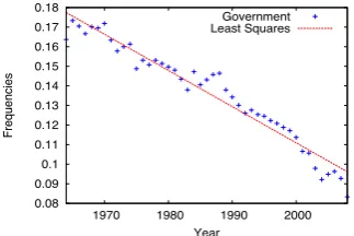
Least Squares. The least squares method is
0
Figure 1:democracy, government, education, welfare, warandterrorismpercentage
In practice we try to determine the longest pe-riod of time in which the data could be fit to a line, imposing that the sum of squares is bond by a small value. For example least squares method applied to the termgovernmentfrom 1968 to 2008 produce the optimal line plotted in Figure 2. The line has the equation: y = 3.807−0.001x. The sum of residuals is less than0.002 (ss= 0.0014), which means that the average variance around the line points is 0.00036. This represents a remark-able fit of data to a line.
Figure 2: Least squares applied to the frequencies for termgovernment
Ratio. It is usual to find in the distribution of
fre-quencies increasing or decreasing sequences. For a definite period of time where a particular direc-tion of growth is observed, we take into account also the rate of growth defined as the ratio be-tween the difference of a three consecutive values:
(xi−xi−1)
(xi+1−xi). In practice we use the growth ratio for
(C1) characterizing a whole period of time and, (C2) for detecting similarities among distributions for different/same terms over the same/different periods.
C1 The same growth rate may characterize a whole period of time. A change in the growth rate may signal the beginning of a new epoch. In Table 4, we report the median growth rate for the termdemocracyover two periods.
year growth rate series average
1850-1900 1.119 1.227 1.227 1.231 1.136 1.23 1.189 1.183
1900-1940 1.218 1.298 1.559 1.69 1.751 1.791 1.802 1.695
Table 4: Growth Rate fordemocracyover two pe-riods
C2 Considering the difference of frequencies of two terms and using the run test we can ob-serve if the growth rate remain the same or changed. In Table 5 we present two runs from two different period of times for the ratio of the differences between the termseducation
anddemocracy. We observe that we have the
same growth ratio pattern in different periods.
year growth rate of difference
1850-1900 +—+—————-+++-+++-+++++–+++++++++–+++
1900-1950 ———————-+–++++++++++++++++++-++++++
Table 5: Growth rates patterns of the difference betweeneducationanddemocracy
Spearman and Kendall Test. Spearman and
0.042
Figure 3:anger, fear, joy, sadness, surpriseandtrustpercentage
give an example of the output of the two tests ap-plied to difference betweengovernment and
wel-fare.
Table 6: Spearman and Kendall test for time vs. difference betweengovernmentandwelfare
0
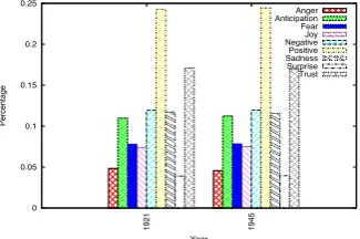
Figure 4: Emotion percentages in 1921 and 1945
The results above show that from the point of view of the relationship between the frequencies
ofgovernmentandwelfare we can clearly
distin-guish four different patterns. There is a strong statistical evidence that the frequencies two terms were correlated in the period 1800-1850 and inde-pendent between 1900-1950.
Before concluding this section we also plot the frequencies of the emotion terms and two exam-ples of emotion blue-print for years 1921 and 1945. The counts were normalized taking into ac-count the emotion words (see Figures 4 and 3).
3.2 Epoch: Decision Procedure
In Section 3.1 we presented the statistical proce-dures we use for epoch determination. Each of these tests is able individually to find non-random changes in the distribution of the frequencies of terms over the years and to find the beginning and the end of the time periods where the same statis-tically relevant pattern - linear, same growth rate, dependency - is observed. However, noticing a change in the distribution is not enough for declar-ing the begin or the end of an epoch. The fact that many of the terms considered are affected by a change in their distribution more or less concomi-tantly must be observed in order to decide on the epoch boundaries. For now, we preferred a conser-vative view therefore in the experiments we car-ried we impose that significantly more than 50% of the terms change their distribution and that the period in which this is happening is at most three years. The algorithm for epoch determination us-ing the tests introduced above is:
Algorithm Epoch Detection
Require: Google N-grams with time info
Ensure: Epoch
1: ApplyW elch0sandRuntest for non-random changes 2: Choose start year and end year spanning several
decades
3: ifnumber of terms positive to line 1 tests in the time in-terval +/- 3 years aroundstart yearandend year≤50%
then
4: gotoline 2 5: end if
6: Apply Least Square, Ratio, Spearman and Kendall 7: ifnumber of terms positive to line 6 tests≤50% then
8: gotoline2 9: end if
At step 6, the order in which the tests are applied is exactly as specified. If Least Square is positive then also the others are positive as well. An so on: if Ratio holds also the last two tests hold. Condi-tion 7 is satisfied if at least Kendall is positive.
4 Experiments
We considered a list of 761 political terms and we applied the decision procedure presented in Sec-tion 3.2. The output of the decision procedure is a set of years around which statistically significant changes in the distribution of frequencies for the majority of the terms considered occur. The epoch identified for the chosen list of terms and the de-cision procedure detailed in Section 3 identified the following 6 epochs epochs between 1800 and 2009, see Table 7.
epoch 1 1800-1860 epoch 4 1950-1975 epoch 2 1860-1900 epoch 5 1975-1999 epoch 3 1900-1950 epoch 6 1999-2009
Table 7: Epochs between 1800-2009
term change year positive test two party system 1975 run, ratio two party system 1999 Welch’s, ratio patriotism 1975 Welch’s, ratio patriotism 1999 Welch’s, squares too big to fail 1975 ratio
too big to fail 1999 squares
Table 8: Statistical significant changes
Table 8 lists a few examples of terms affected by a statistical change at epoch boundaries. In Table 9 we present the number of terms which changed their distribution for each boundary, on the second column the absolute value and on the third column the percentage relative to the total number of terms considered, 761. We can see that the number of terms which are positive to statistical tests varies substantially. However, it is not by chance that the changes occur.
year number of terms percentage
1860 518 68%
1900 491 64%
1950 579 76%
1975 682 89%
1999 607 78%
Table 9: The number of terms defining an epoch
There is a tolerance of a couple of years around the boundaries. For example, if a term’s distri-bution changes +/-3 years around 1975, then this
change is considered for epoch boundary delim-itation. Especially in the last 60 years, it seems that the changes occur more frequently and they are more clearly delimited. During these times, the changes between two different trends occur within a couple of year in the great majority of cases. The dynamic of change is different in the nineteenth century, when it is more likely to observe a buffer zone for several years. In the buffer zone, the dis-tribution around a mean value is quasi normal.
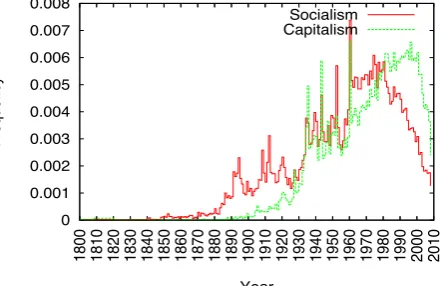
In fact, by running Spearman and Kendall tests we discovered interesting dependencies between the distribution of certain terms and the time line. We computed the differences between the frequen-cies of pair of terms. For example, for the pair
so-cialismandcapitalismthe results of the statistical
tests show a strong correlation within each epoch, see Table 10 and Figure 5.
0 0.001 0.002 0.003 0.004 0.005 0.006 0.007 0.008
1800 1810 1820 1830 1840 1850 1860 1870 1880 1890 1900 1910 1920 1930 1940 1950 1960 1970 1980 1990 2000 2010
Frequency
Year
Socialism Capitalism
Figure 5: Socialism vs. Capitalism through the epochs
epoch Spearman Test Kendall Test Dependent
1800-1860 0.9741 0.9138 yes
1860-1900 0.9402 0.8429 yes
1900-1950 0.2073 0.0108 no
1950-1975 0.2210 0.0962 no
1975 -1999 -0.9762 -0.8977 yes
1999-2009 -0.945 -0.8891 yes
Table 10: socialism vs. capitalism through the epochs
anger anticipation disgust fear
3914 9390 2448 6519
joy sadness surprise trust
6053 9892 3173 12082
term 1800-1860 1860-1900 1900-1950 1950-1975 1975-1999 1999-2009
anger 0.0546 0.0540 0.0491 0.0467 0.0458 0.0455
anticipation 0.1093 0.1112 0.1129 0.1157 0.1178 0.1158
disgust 0.0358 0.0344 0.0303 0.0282 0.0283 0.0287
fear 0.0813 0.0813 0.0786 0.0813 0.0819 0.0769
joy 0.0842 0.0818 0.0771 0.0736 0.0693 0.0706
sadness 0.1149 0.1224 0.1206 0.1216 0.1240 0.1188
surprise 0.0395 0.0421 0.0405 0.0388 0.371 0.0378
trust 0.1680 0.1680 0.1722 0.1791 0.1775 0.1672
Table 12: The average of emotion frequencies over the epochs
Figure 6: 10-fold validation
To each epoch an emotional blueprint can be at-tached. An emotional blueprint is obtained by tak-ing into consideration the emotion denottak-ing terms. There are 7 emotion words; anger, anticipation,
disgust,fear,joy,sadness,surprise,trustand two
opinion words,negativeandpositive. The corpus we consider in this section is the part of Google 5-grams in which each 5-gram contains at least an emotion word. In Table 11 we present their distri-bution in Google-gram corpus.
The epoch characterization task consists in us-ing the epochs as categories and assignus-ing an un-seen sample covering a continuos, but unknown, period of time to one of the categories. For the ex-periments in this paper, we used the average values of each emotion term computed over the epochs as epoch blue print, thus each epoch is characterized by an unique value for each emotion term, see Ta-ble 12.
For evaluation we used a k-fold cross valida-tion approach. The k-partivalida-tions were obtained by
choosing randomly for each occurrence in google corpus its partition, so in average each partition had an equal number of terms. The training was carried onk−1 partitions and tested on a single partition, thus there are kindependent evaluation experiments. The training k−1 partitions were joined into an unique corpus which was split into epochs and for each epoch we computed the av-erage for each emotion term. The test partition, the k-partition was split in ten contiguous sub-partitions. For each test sub-partition, the aver-age of the emotion terms was computed and com-pared against the averages from training corpus to find the most similar ones, resulting in10k exper-iments (see Figure 6).
experiment first run second run third run fourth run fifth run
all occurrences squares sum 46% 51% 46% 48% 50%
all occurrences best guess 60% 56% 60% 59% 60%
co-occurrences squares sum 53% 58% 59% 57% 59%
co-occurrences best guess 65% 69% 67% 66% 66%
Table 13: 5-partition cross-validation results
for each particular epoch. The category assigned is the one with the least sum of squares. The second method compares the averages computed over the training for each epoch and chooses a representa-tive for each epoch, let us call it best guess. The test sample compares only the averages against the best guess for each epoch and it is assigned to the epoch which has the closest best guess.
To measure the accuracy, we simply count how many times there was only one epoch chosen and that it was indeed the correct one. The figures re-ported in Table 13 represent the accuracy, as all the sub-partitions were checked and consequently the recall was 1. The last two experiments we car-ried out on considered political terms. Instead of considering all occurrences of the emotion terms inside a particular epoch, we considered only the co-occurrences of the emotion words with a set of political terms. For this purpose we chose a set of 20 from the list of 761 of political terms con-sidered: capitalism, community, common good,
democracy, education, free market, government,
heresy hunting, individual rights, justice, middle
class, money, nepotism, politics, public interest,
savings,socialism,social system,technology, and
war. The averages for each corpus, training and test respectively, were computed only for these terms and the two approaches above, squares sum and best guess were applied.
In order to understand weather the results above are informative, we run a simple baseline over the same data. The baseline decision was to consider for each subpartion a random epoch. The accuracy of the baseline is around 15%.
5 Conclusion and Further Research
The possibility to analyze automatically the changes over the time in the usage of certain terms is an open window into sociological studies car-ried from a language perspective with computa-tional methods.
During the experiments, some interesting re-search directions have been revealed. Firstly, al-though we made no attempt here to make the
con-nection between certain changes and real histori-cal events, it seemed that this was indeed possi-ble. Sharply distinctive changes are observed for certain terms around global war dates. Secondly, while we used the ratio as a parameter which may signal a change, we carried no analyses on the ty-pology of rates themselves. Such analyses may bring to light patterns into the dynamic of inter-ests within a society. Thirdly, the methodology we presented can be easily used for prediction. Such studies could predict future changes. A striking example is represented by the covariance between socialism and capitalism, which seemed to indi-cate the collapse of political regimes in East Eu-rope several years before it actually happened, see Figure 5. We plan to investigate further the distri-bution of terms over the time going in the direc-tions above.
References
A. Bj¨orck. 1996. Numerical Methods for Least Squares Problems. SIAM: Society for Industrial and Applied Mathematics.
J. D. Gibbons and S. Chakraborti. 1992. Nonparamet-ric Statistical Inference. CRC Press.
P. Joula. 2012. Using the google ngram corpus to mea-sure cultural complexity. InProceedings of Digital Humanities, University of Hamburg, July.
B. Lindgren. 1993. Statistical Theory. Chapman and Hall/CRC.
J. B. Michel, Y.K. Shen, A.P. Aiden, A. Veres , M. K. Gray, J.P. Pickett, D. Hoiberg, D. Clancy, P. Norvig, J. Orwant, M. A. Nowak S. Pinker, and E.L. Aiden. 2011. Quantitive analysis of culture using millions of digitized books. Science, 331(6014):176–182, January.
Saif Mohammad and Peter Turney. 2010. Emotions evoked by common words and phrases: Using me-chanical turk to create an emotion lexicon. In Pro-ceedings of the NAACL HLT 2010 Workshop on Computational Approaches to Analysis and Genera-tion of EmoGenera-tion in Text, pages 26–34, Los Angeles, CA, June. Association for Computational Linguis-tics.
B. Pang and L. Lee. 2008. Opinion mining and senti-ment analysis. Foundations and Trends in Informa-tion Retrieval, 2(1-2):1–135.
S. Sawilowsky. 2001. Fermat, schubert, einstein, and behrens-fisher: The probable difference between two means whenσ2
1 6=σ22. Journal of Modern
Ap-plied Statistical Methods, 1(2):461–472.
C. Strapparava and R. Mihalcea. 2007. SemEval-2007 task 14: Affective Text. InProceedings of SemEval-2007, Prague, Czech Republic, June.
C. Strapparava and A. Valitutti. 2004. Wordnet-affect: an affective extension of wordnet. InProceedings of the 4th International Conference on Language Re-sources and Evaluation, Lisbon.
X. Wang and A. Mccallum. 2006. Topics over time: A non markov continuos-time model of topical trends. In Proceedings of KDD-06, Philadelphia, Pennsyl-vania, August.
C. Wang, D. Blei, and D. Heckerman. 2008. Continous time dynamic topic models. InProceedings of the International Conference on Machine Learning.