Theoretical analysis and optimization of circular patch microstrip antenna

© 2015, IRJET.NET- All Rights Reserved

Page 1675

Theoretical analysis and optimization of circular patch

microstrip antenna

Monika Bhatnagar

Assistant Professor, I.T.S Engg College, Gr.NOIDA,

monikabhatnagar06@gmail.com

Abstract -

Key Words:

Microstrip antenn; circular sector microstrip

1. INTRODUCTION

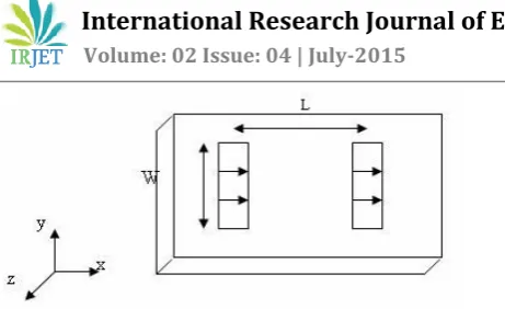
The first appearance of the concepts of microstrip antennas dates back to 1953, but during the 70 years that the first projects have emerged [1], then the antennas have benefited from the development of printed circuit boards to be used widely in the field of wireless. The patch antennas have several advantages that have attracted the industrial field: low profile, low weight, small volume and low cost manufacturing. However, they have some disadvantages: Low bandwidth, low power and low gain. A microstrip antenna typically consists of a conducting plane called patch printed on a substrate having a ground plane. The patch can be of any shape: rectangular, circular and annular [7]. The antenna can be excited by a coaxial cable, a microstrip line or coupled by aperture or proximity. The excitation guide the electromagnetic energy source to the patch and this generates negative charges around the feed point and positive charges of the other part of the patch. This difference in charge creates electric fields in the antenna; the electric fields are responsible for the radiation of the patch antenna as shown in Figure 1.

There is three types of waves radiated [2]: The first part is emitted into space is the "useful" that is responsible of radiation. The second part is diffracted waves and back into space between the patch and the ground plane that contributes to the power transmission. Finally, the third part of the wave remains trapped in the dielectric substrate by total.

here. reflection on the separation surface air-dielectric. The waves trapped in the substrate are generally undesirable.

In this paper we study the CSMA; we start by outlining some theoretical notions about the patch antennas: the various methods for analyzing antennas, resonant frequency and circular polarization. Second, the design of CSMA will be exposed through the design criteria of each part: substrate, patch, feeding mode. Finally simulations will be launched using HFSS tool and the results will be compared with literature and analyzed.

Figure 1. Electrical field radiated by a microstrip antenna

2. THEORY

The methods of analysis of antennas have been developed to help understand their principles, to predict their radiation characteristics and to reduce costs for design and manufacturing. The most used methods are [1] [4] [5]: Model of the transmission line, the model of the resonant cavity and numerical methods that include the integral equations and the method of moments. In this article we will give a definition of these methods, the method of the resonant cavity will be detailed and applied later to CSMA.

A. Model of the transmission line

© 2015, IRJET.NET- All Rights Reserved

Page 1676

of a rectangular element

B. Numerical methods

The most used numerical methods in electromagnetism are:

1) The finite elements:

The finite element method is applied to microwave devices of any shape. It is based on solving Maxwell's equations and the geometric description of the structure in the form of a mesh. This method consist to divide the space into small homogeneous elements but practically very variable in size. The advantage of the finite element method is that the tetrahedral shape and size variation of the elementary cells characterizing the volume discretized provides great flexibility. This method allows the simulation of complex geometric structures, but with strong mathematical tools.

2) Matrix of Transmission Lines TLM:

The method of the matrix of transmission lines TLM discretizes the fields and currents of the studied structure into small elements. Each of these elements is considered as a set of transmission line and the calculations are done directly in the time domain. The advantage of this method is the simple formulation that does not depend much on the geometry of the structure studied; it is easy to handle complex structures composed of several materials, and particularly suitable for the analysis of multilayer planar structures.

3) The finite difference:

The finite difference method calculates in every moment of the discrete space the electromagnetic field components in each unit cell of three-dimensional volume. We Apply the Fourier transform to the time response for the frequency response of the system. The main advantage of this method is the simplicity of its formula; the calculation is then made in the time domain over a wide frequency band. The computation time grows linearly with the number of unknowns (which is not the case for the finite element method). But its main drawback is the fact that the mesh of the structure must be uniform and is therefore not suitable for the treatment of devices containing elements with very different orders of magnitude.

4) The method of moments:

Using the method of moments in electromagnetic problems has been developed for the first time by Newman, it is a method of solving integral equations that reduces them into a system of linear equations applied to

planar structures and quasi-planar structure of the 2-D. To use this method, we must break down the structure studied in several parts or cells. The numerical solution of Maxwell's equations of the structure studied can write the electric or magnetic fields according to a sum of induced currents. Calculating the current distribution measured on each section by cancellation of tangential electric fields provides the [Z]. In the method of moments, the integral equation is reduced to a set of linear algebraic equations of the form: [Z] • [I] = [V]. The impedance matrix [Z] is calculated from the integral equations. It will excite the structure with the voltage vector [V] and then the current vector [I] will be calculated. Once the current calculated for each element, the electric and magnetic fields are determined.

C. The model of the resonant cavity:

This model is more accurate and complex. As the model of the transmission line provides a good physical interpretation. For the study of other geometrical shapes of the radiating element, the model of the cavity is more suitable. This applies in the region limited by the metal surface of the patch and the associated ground plane. The main bases of this model for very thin substrates are:

• The fields inside the cavity do not change depending on z (δ \ δz = 0);

• The direction of the electric field is along z and the magnetic field is transverse.

• We assume that the side walls are magnetic walls (H = 0) and the top and bottom electric walls (nxe = 0). n is a unit vector normal to the walls of the cavity.

From these observations we can conclude that only the component Ez of E field is not zero. From Maxwell's equations we find that Ez satisfies the following equation [5]:

As k2 = ω2µ0ε0ε and J the current density of the excitation of the antenna (coaxial cable or microstrip line). The solution of equation (1) is:

Amn is the amplitude coefficient for a mode or an

eigenvalue ψmn. The eigenvalues are the solutions of the

equation:

Note that these eigenvalues depend on the form is the size of the patch but not the parameters of the substrate.

To find the expression of ψmn, Ez is replaced in (1) by

© 2015, IRJET.NET- All Rights Reserved

Page 1677

So the expression of Ez becomes:

We can deduce the expression of the fields H:

The expression of the electric field (5) is expressed in terms of eigenvalues that depend on the shape of the patch dimensions. So for a patch with any shape, the calculation of the electric field is to find the proper value on this form. Several studies have been conducted to find the eigenvalues for a given form of the patch. In [5], [6] and [7] found the expression values for a patch antenna with circular, triangular, ring and other forms.

Applying the model of the resonant cavity on a CSMA: To study the antenna (see Figure 3), we model it by a cavity based on circular sectors, its radius is equal to the patch and "filled" with a dielectric permittivity ε and height h equals that of the substrate. The vertical walls of the cavity walls are assumed to be magnetic on which the continuity conditions are: EN=0 and HT=0. The excitation of the antenna produces inside this cavity field E directed along the z axis and a field H which is in the xy plane (TM mode). We recall the general expression for a patch antenna according to the model cavity:

The eigenvalue for a circular sector is available for sectors at an angle α which divide π. The expression of the eigenvalue in this case is [5]:

υ = nπ / α, Jυ is the Bessel function of order υ and kmυ checks:

So if we replace in (5) by (7) and we do the calculations of integrals we find the expression of the field Ez [8]:

(9) The resonance occurs for k = kmυ

To calculate the resonant frequency, we must first solve

the equation: J’ (kmυa) = 0, in [7] we find the solution of this equation for each type of patch is called the normal frequency of resonance. The latter must be multiplied

by: Finally, to find the resonant frequency. To calculate the resonant frequency of CSMA: In [7], the normalized frequency for CSMA is 3.054. After

multiplication by we found theoretical resonance frequency: fth=2.28 GHz this result will be confirmed by simulating the CSMA in HFSS.

D. Circular polarization:

The polarization of an antenna is determined by the wave radiated in a given direction, it is identical to the direction of the electric field. The instantaneous electric field vector traces a figure in time. This figure is usually an ellipse which has special cases. If the path of the electric field vector follows a line, the antenna is said to be linearly polarized. If the electric field vector rotates in a circle, it is called circularly polarized as shown in Figure 4 [9]. To characterize the polarization, the axial ratio is used. It is defined by:

© 2015, IRJET.NET- All Rights Reserved

Page 1678

Linear polarization or linear (T → ∞ or T = 0): obtained when the field is parallel to a direction in time: the ellipse becomes a straight line.

Circular polarization (T = 1) right or left: when both fields have the same amplitudes (Eθm = Eφm) and vibrate in phase quadrature: the ellipse becomes a circle.

In this paper, we are interested to the circular polarization. Almost to the circular polarization axial ratio should not exceed 3 dB. The calculation of axial ratio will be done on HFSS to define the polarization of CSMA. We will be interested by circular polarization because the error rate is reduced and interferences are attenuated multi-path [14] [15].

3. ANTENNA DESIGN

To achieve an optimal design of the patch antenna, it is necessary to study each part of the antenna: substrate, patch shape, feeding and dimensions of the antenna. 1) Choice of substrate:

The substrate is often a dielectric with a permittivity of between 2.1 and 25. Substrates based on polytetrafluoroethylene (PTFE) are widely used because of their electrical and mechanical characteristics. [1] In this context, the substrate must have a minimum cost and an average permittivity in order to have a miniature antenna with a minimum loss. The chosen substrate is RO3200 which is a combination PTFE /ceramic with glass fabric reinforcement, the permittivity is εr = 10.2 and tangential loss is tanδ = 0.0035.

2) Choice of the shape of the patch

The radiating element can have several geometric shapes, the rectangle is the most studied since it is simple for understanding the mechanisms of radiation of patch antennas. Circular patch antennas are often treated, however, little effort has been made to study the circular sector patch antennas, the latter type can solve some of geometrics constraints and allows for miniature antennas. [7]

In this paper, the patch shape: circular sector with and angle α = 90° was treated in this article for the design of our antenna.

3) Choice of type of feeding:

Based on comparison [5] between different types of feed we can conclude that:

• The feeding microstrip line and coaxial cable feed are easy to implement, however, this type of power generating spurious radiation which affects the radiation pattern.

• The power coupled by proximity and power coupled opening offer greater bandwidth and better radiation pattern by cons are not easy to implement.

In this article we have chosen to feed our antenna via a microstrip line and secondly via a coaxial cable. We will compare the results for these two modes of feeding. 4) Dimension of the antenna:

© 2015, IRJET.NET- All Rights Reserved

Page 1679

4. RESULTS AND DISCUSSION

Antennas studied in this paper are: Antenna 1: circular sector patch antenna fed by a coaxial cable. Antenna 2: circular sector patch antenna fed by a microstrip line. We used the tool HFSS 9 for the study of these antennas and this for the following analysis:

• First analysis: We studied the impact of changing the shape and dimensions of the patch for substrates with low and high permittivity. Since the rectangular patch antennas are the most studied [11] [12] [13], we referred to studies conducted on this type of antenna to compare with our antenna.

• Second analysis: We studied the CSMA for two feeding modes: coaxial and microstrip line fed. Results are compared with the experiment realized in [8].

• Third analysis: Polarization of antenna 1 and 2 are analyzed.

In table 2, dimensions of the patch studied are presented, its surface, the permittivity of the substrate and its thickness. For each antenna the resonance frequency is calculated or reported from literature [11][12]. Following observation are confirmed: The substrate of high permittivity decreases the resonant frequencies. The increase in the surface of the patch reduces the frequency of resonance and for the circular sector patch, for surface 3. 14cm2 the same resonant frequency could be obtained using a rectangular patch of surface 6cm2. Hence the possibility of reducing the size of the patch antenna using a circular sector of using the rectangular surface. On the other hand by comparing a rectangular patch antenna and an CSMA having the same dimensions and using the same substrate, the CSMA has a resonant frequency lower.

The advantage of using a circular sector becomes more important in tracing the reflection coefficient of our antennas 1 and 2 (Figure 5). This figure shows that the proposed antenna can radiate with a good reflection coefficient (better than -10 dB) for frequencies 2.20; 2.60 and 3.80 GHz for the antenna 1 and the frequencies 2.17, 2.48 and 3.76 GHz for the antenna 2.

© 2015, IRJET.NET- All Rights Reserved

Page 1680

antennas for frequencies 2.17 GHz, 2.6 GHz and 3.8 GHz in horizontal plane (Phi = 0 °) and vertical (Phi = 90 °). Figures 6 and 7 represent an acceptable radiation pattern for the two antennas, however, for the diagrams obtained for the 3.8GHz frequency are not directivesImpact of changing the shape, dimensions of the patch and substrate Last analysis is to determine the polarization of the antennas studied We have covered the literature to define the different methods for generating a circular polarization. The Classical method is to feed an antenna by two points 90 ° phased or adding perturbations at the patch (slit hole). [9][10][14-16]

The axial ratio was calculated at the frequency 2.2 and 2. 17 GHz. For antenna 1 and 2, we noted that the two antennas show the same axial ratio for the two feeding modes, which was already planned since the polarization is independent of feeding mode. Figure 9 shows the values of axial ratio for θ between [-90, 90 °].

As explained in (II.4) circular polarization corresponds to axial ratio lower than 3 dB. From the diagram, the antenna has a circular polarization for θ in the interval [-45, 45 °]. This result is important in the sense that we could obtain a circular polarization with a single antenna and using a single fed without the need to add a perturbation to patch or add a second fed.

5. CONCLUSION

We have presented a theoretical overview on methods for analysis of patch antennas and the main principles (structure of the antenna, the choice of fed, the patch and the substrate) to design a patch antenna. A rigorous theoretical study was projected on the CSMA. Cavity model was applied on the proposed antenna to calculate radiation fields and resonant frequency.

The theoretical study of antenna CSMA, launched in HFSS simulations and comparing the results with those available in the literature have shown that the proposed antenna repent the following advantages: low-cost, easy to manufacture, dimensions miniature circular polarization, can operate in two bands and may be offered especially for mobile applications.

As perspectives for this work, it is possible to reproduce and confirm these results by making the antenna.

REFERENCES

[1] K.R. Carver ET J.W.Mink “Microstrip Antenna Technology” IEEE Transactions on Antennas and Propagations Vol. ap-29, no. 1, January 1981

[2] L. Zenkouar «Contribution to the dynamic study in the space domain of microstrip lines on high permittivity substrate» PhD thesis, University of Liege 1996 [3] Paul F. Combes « Microwave: passive circuits,

propagation, antennas» Edition DUNOD 1997.

© 2015, IRJET.NET- All Rights Reserved

Page 1681

Antenna Design Handbook” Artech House 2001 [6] Y.Lo, D.Solomon, W.F.Richards “Theory and

Experiment on Microstrip Antennas” IEEE Transactions on Antennas and Propagation, VOL.AP 27 NO2 March 1979

[7] W.F.Richard J.D Ou S.A.Long “A Theoretical and Experimental Investigation of Annular, Annular Sector and Circular Sector Microstrip Antennas” IEEE Transactions On Prograpation Vol AP32 No8 August 1984

[8] V K Tiwari, A.Kimothi, D.Bhatnagar, J.S Saini, V.K Saxena “Theoretical Analysis on Circular Sector Microstrip Antennas” Indian Journal of Radio and Space Physics Vol 35 April 2006 pp 133-138

[9] M. Shakeeb “Circularly Polarized Antenna” Tehsis Master of Applied Science at Concordia University Quebec, Canada 2010

[10] M. Diblanc “Developpement du concept de l’ antenne { resonateur BIE pour la generation de la polarisation circulaire” These doctorat de l’ Université de Limoges 2006.

[11] D.Shaubert D.M.Pozar A.Adrian “Effect of Microstrip Antenna Substrate Thickness and Permittivity: Comparison of Theories with experiment” IEEE Transactions on Antennas and Propagation, Vol. 31, no. 6, June 1989

[12] W. Dearnley, F. Barel “A Comparison of Models to Determine the Resonant Ekequencies of a Rectangular Microstrip Antenna” IEEE Transactions on Antennas and Propagation, Vol. 37, no. 1, January 1989

[13] F.Harrou, A.Tassadit, B.Bouyeddou “Analysis and Synthesis of Rectangular Microstrip Antenna” Journal of Modelling and Simulation of Systems Vol.1-2010 pp. 34-39

[14] S.Maddio, A.Cidronali, Member and G.Manes “A New Design Method for Single-Feed Circular Polarization Microstrip Antenna With an Arbitrary Impedance Matching Condition” IEEE Transactions on Antennas and Propagation, vol. 59, no. 2, February 2011 [15] J.Sze, W.Chen ”Axial-Ratio-Bandwidth Enhancement