Regularization of an initial inverse problem for a biharmonic equation

R E S E A R C H

Open Access

Regularization of an initial inverse problem

for a biharmonic equation

Hua Quoc Nam Danh

_{, Donal O’Regan}

_{, Van Au Vo}

_{, Binh Thanh Tran}

_{and Can Huu Nguyen}

*_{Correspondence:} [email protected] 6_{Applied Analysis Research Group,}

Faculty of Mathematics and Statistics, Ton Duc Thang University, Ho Chi Minh City, Vietnam Full list of author information is available at the end of the article

Abstract

In this paper, we consider the problem of finding the initial distribution for the linear inhomogeneous biharmonic equation. The problem is severely ill-posed in the sense of Hadamard. In order to obtain a stable numerical solution, we propose two regularization methods to solve the problem. We show rigourously, with error estimates provided, that the corresponding regularized solutions converge to the true solution strongly inL2_{uniformly with respect to the space coordinate under} somea prioriassumptions on the solution. Finally, in order to increase the significance of the study, numerical results are presented and discussed illustrating the theoretical findings in terms of accuracy and stability.

MSC: 35K99; 47J06; 47H10; 35K05

Keywords: Backward problem; Biharmonic equation; Polyharmonic problem; Regularization method; Error estimate

1 Introduction

In this paper, we consider the non-homogeneous biharmonic equation

⎧ ⎪ ⎪ ⎪ ⎪ ⎪ ⎨ ⎪ ⎪ ⎪ ⎪ ⎪ ⎩

2u=∂4u

∂y4 + 2 ∂ 4_u

∂y2_∂x2 +∂ 4_u

∂x4 =ρ(y,x), inQL:= (0,L)×Ω, u(y,x) =u(y,x) = 0, onΣL:= (0,L)×∂Ω,

u(L,x) =g(x), ∂_∂u_yu(L,x) = 0, inΩ,

u(L,x) =h(x), ∂u

∂y (L,x) = 0, inΩ,

(1.1)

whereΩ⊂Rd,d≥1 is an open bounded domain with a smooth boundary∂Ω, and the linear source functionρ∈L∞(0,L;L2(Ω)). In practice, the datag,h∈L2(Ω) are noisy and are represented by the observation datagα_,hα_∈L2_{(Ω) satisfying}

gα_–g

L2_(Ω)≤α, hα–h_L2_(Ω)≤α; (1.2)

hereα> 0 is a small positive number representing the level of noise.

There are many papers on different methods for approximating solutions to boundary value problems for elliptic partial differential equations and most are centered on second order equations where maximum principles are used to obtain asymptotic estimates for the error [1–5,7,8,11,13–15,17–19]. The theory for elliptic equations of order greater

than two is less developed [8] (note that such equations arise in physics and in engineering design and they also appear naturally in many areas of mathematics, including conformal geometry, and nonlinear elasticity [1,4,5]).

The prototypical example of a higher-order elliptic operator, well known from the the-ory of elasticity, is the biharmonic2=() =∇4, and a more general example is the polyharmonic operatorp= (...)

ptimes

,p> 2. The biharmonic equation arises in many

engineering applications such as the deformation of thin plates, the motion of fluids, free boundary problems, nonlinear elasticity and for historical details we refer the reader to [2,3,7,14] (for a more elaborate history of the biharmonic problem and the relation with elasticity from an engineering point of view we refer the reader to the survey of Meleshko [11]).

In 1928, Covrant et al. [6] posed a difference analog for the first boundary value problem for the homogeneous biharmonic equation

Lu=

∂2u

∂y2 + ∂2u

∂x2 2

= 0 (1.3)

and proved that the approximate solutions converge to the exact solution as the mesh is refined (however, no estimates for the error were given). In [10], the authors obtained necessary and sufficient conditions for existence of a solution for the biharmonic equation (1.3) in a rectangular domain [0,π]×[0,L] in the spaceL2_{(0,π). In [9] using a nonlocal}

boundary value problem method, convergence of regularized approximation with a priori parameter choice was proven, provided data noise level tends to zero (however, the authors did not investigate error estimates). The method of nonlocal boundary value problems for second order elliptic equations was used by several authors (see [13,15,17–19]). There are many papers on the linear homogeneous case for the biharmonic equation, but, how-ever, very little is known on regularization theory and numerical simulation for the linear inhomogeneous case. Our main aim in this paper is to discuss regularized solutions for problem (1.1). Using the Fourier truncation method introduced in [16], we propose the regularized solution and give an error estimate.

The paper is organized as follows. In Sect.2, the formulation of the problem and its ill-posed property are given. In Sect.3, stability estimates are proved under a priori condi-tions on the solution. Numerical results are presented and discussed in Sect.4and, finally, conclusions are summarized in Sect.5.

2 Preliminaries

2.1 Notations and assumptions

We begin this section by introducing some notations and assumptions that are needed for our analysis in the next sections.

Definition 2.1 Without loss of generality, we assume that –has the eigenvalues λm

(m∈N∗):

0 <λ1≤λ2≤λ3≤ · · · ∞, (2.1)

Definition 2.2(Hilbert scale space, see [12]) The Hilbert scale spaceHp_{, (p> 0) defined}

by

Hp_:=

f ∈L2(Ω) :

∞

m=1

λ2_mpf,ξm(x)

2

L2_(Ω)≤ ∞

, (2.2)

is equipped with the norm defined by

f2_Hp=

∞

m=1

λ2_mpf,ξm(x)

L2_(Ω)

2

≤ ∞. (2.3)

For a Hilbert spaceX, we denote byLp_{(0,L;X) (respectively,C([0,L];X)) the Banach space}

of measurable (respectively, continuous) functionsf : [0,L]→X, such that

f_Lp_(0,L;X)=

L

0

f(y)p_Xdy

1/p

<∞, 1≤p<∞,

f_L∞_(0,L;X)=ess sup 0≤y≤L

f(y)_X<∞, p=∞,

respectively,

fC([0,L];X)= sup 0≤y≤L

f(y)_X<∞.

Throughout this paper, the functionρis perturbed so as to contain errors in the form of noisyρα_∈L∞_(0,L;L2_{(Ω)) satisfying}

ρα–ρ_L∞

(0,L;L2_(Ω))≤α. (2.4)

2.2 Mild solution and ill-posed of problem (1.1)

The solution to problem (1.1) can be represented in the form of an expansion in the or-thogonal series

u(y,x) =

∞

m=1

um(y)ξm(x), withum(y) =

u(y,x),ξm(x)

L2_(Ω). (2.5)

By considering that the series (2.5) converges and allows a term by term differentiation (the required number of times), we construct a formal solution to the problem. We obtain the problems

⎧ ⎪ ⎪ ⎨ ⎪ ⎪ ⎩

u(4)m(y) – 2λmum(y) +λm2um(y) =ρm(y), y∈(0,L), um(L) =gm, um(L) = 0,

u_m(L) –λmum(L) =hm, um(L) –λmum(L) = 0.

(2.6)

Heregm,hmandρm(y) are Fourier coefficients of the expansion according to the

orthonor-mal basis{ξm(x)}m∈N∗of the functionsg(x),h(x) andρ(y,x), respectively:

g(x) =

∞

m=1

gmξm(x), h(x) =

∞

m=1

ρ(y,x) =

∞

m=1

ρm(y)ξm(x).

By direct calculation, the solution to problem (2.6) has the form

um(y) =coshλm(L–y)

Substituting the result into (2.5), we obtain the formal solution to problem (1.1).

Next, we give an example which shows that the solution of problem (1.1) does not de-pend continuously on the final data.

and it follows that

Hence, we deduce that

uj_L∞_(0,L;L2_(Ω))=ess sup

Thus our problem is ill-posed in the Hadamard sense in theL2(Ω)-norm.

3 Regularization and error estimate

In order to obtain stable numerical solutions, we propose two regularization methods to solve the problem. As was shown in the previous section, for the linear biharmonic problem (1.1), its solution (true solution) can be represented as an integral equation which contains some instability terms. Indeed, we find that the four functions

cosh(λmz),sinh(λmz), z> 0,

in (2.7) are unbounded, as functions of the variablem, fory∈(0,L). Consequently, small errors in high frequency components can blow up and completely destroy the solution fory∈(0,L). A natural idea to stabilize the problem is to eliminate all high frequencies (truncation method) or to replace them by a bounded approximation (quasi-boundary value method). We introduce two bounded operators as follows:

where

Iγ(α)

L,m =

1 +γ(α)λme√λmL–1_{, ∀m∈N}∗_,

andγ(α) > 0is the parameter regularization which satisfies

lim

α→0+γ(α) = 0. (3.2)

• Forf ∈C([0,L];L2(Ω)), we define

BMα_{f(y,x) =}

m∈T† α

f(y,x),ξm(x)

L2_(Ω)ξm(x), (3.3)

where

T† α:=

m∈N∗|λm≤Mα

,

andMα> 0is the parameter regularization which satisfies

lim

α→0+Mα= +∞. (3.4)

3.1 The main results

3.1.1 Result for quasi-boundary value method

Let us consider the following well-posed problem:

⎧ ⎪ ⎪ ⎪ ⎪ ⎪ ⎨ ⎪ ⎪ ⎪ ⎪ ⎪ ⎩

2uγ(α)_=Qγ(α)_ρα_{(y,x), inQ}

L,

uγ(α)_=uγ(α)_{= 0, onΣ}

L,

uγ(α)_{(L,x) =Q}γ(α)_gα_(x), ∂uα

∂y(L,x) = 0, inΩ,

uγ(α)_{(L,x) =Q}γ(α)_hα_(x), ∂uγ(α)

∂y (L,x) = 0, inΩ.

(3.5)

Theorem 3.1((QBV) method) Assume that the exact solution u of (1.1)satisfies

u_L∞_(0,L;Hp+1_(Ω))≤E₁, (3.6)

where p,E1are positive constants.Chooseγ(α)∈(0, 1)such that ⎧

⎨ ⎩

limα→0+γ(α) = 0,

limα→0+ α

γ(α)=finite.

(3.7)

Then the estimate

uγ(α)(y,·) –u(y,·)_L2_(Ω)≤

C(λ1,L) log( L

γ(α))

α γ(α)+E1

(3.8)

holds.

Remark3.1 From condition (3.7), if we chooseγ(α) =αk_{for somek∈(0, 1), then the error}

estimate in (3.8) is of order_logα1–k

(L αk)

3.1.2 Result for truncation method

Next, we propose a second regularized solutionuα_{solving the following problem:}

⎧ ⎪ ⎪ ⎪ ⎪ ⎪ ⎨ ⎪ ⎪ ⎪ ⎪ ⎪ ⎩

2_uα_=BMα_ρα_{(y,x), inQL,}

uα_=uα_{= 0, onΣ}

L,

uα_{(L,x) =B}Mα_gα_(x), ∂uα

∂y(L,x) = 0, inΩ,

uα_{(L,x) =B}Mα_hα_(x), ∂uα

∂y (L,x) = 0, inΩ.

(3.9)

Theorem 3.2 ((TR)method).Suppose that the problem(1.1)has a solution u satisfying

u_L∞_(0,L;Hp_(Ω))≤E₂, (3.10)

for some known constant E2> 0.Assume that we can choose Mα> 0such that

⎧ ⎨ ⎩

limα→0+M_α= +∞,

limα→0+_αeL

√

Mα_{= 0.}

(3.11)

Then

_uα

(y,·) –u(y,·)_L2_(Ω)≤Ce

√

MαL_α+ E2

Mαp

. (3.12)

Remark3.2 Let us chooseMα=_L12log2(α–), for some∈(0, 1). Then the hypothesis

lim α→0+αe

L√Mα_{= 0,}

is fulfilled and (3.12) is of order

max

α1–; 1

log2p(α–₎

, p∈N∗. (3.13)

Theorem 3.3(EstimateHp_{) Let us choose M}

α> 0such thatlimα→0+M_α=∞and

lim α→0+αM

p

αe

√

MαL_<∞_{. (3.14)}

Assume further that the problem (1.1) has a unique exact solution u satisfying u ∈ L∞_(0,L;Hp+q_{),for p,q> 0.Then,for all y∈[0,L],we have}

uα(y,·) –u(y,·)_Hp_(Ω) ≤C(λ1,L)Mpαe

√

MαL_α+M–q

α uL∞(0,L;Hp+q_(Ω)). (3.15)

Remark3.3 Let anyχ∈(0, 1). We choose

Mα=

log2(α–χ₎

Then condition (3.14) is satisfied asα→0+_{and the right-hand side of (3.15) is of order}

max

log2pα–χα1–χ; 1

log2q(α–χ₎

, p,q> 0. (3.16)

3.2 Proof of Theorem3.1

Problem (3.5) can be rewritten as the following integral equation:

uγ(α)(y,x) =

∞

m=1

coshγ(α)λm(L–y)

g_mα ξm(x)

+

∞

m=1

(L–y)sinhγ(α)(√λm(L–y))

2√λm

hα

m

ξm(x)

+

∞

m=1

L

y

(σ–y)coshγ(α)₍√_λ

m(σ–y))

2λm

ρ_mα(σ)dσ

ξm(x)

+

∞

m=1

L

y

sinhγ(α)(√λm(σ–y))

2λm

√ λm

ρ_mα(σ)dσ

ξm(x), (3.17)

where we define the operators forz> 0

coshγ(α)_(λ

mz) :=I

γ(α)

L,m cosh(

λmz), (3.18)

sinhγ(α)(λmz) :=I_Lγ_,m(α)sinh(λmz), (3.19)

and

gα

m=

gα_(x),ξ

m(x)

L2_(Ω), hαm=

hα_(x),ξ

m(x)

L2_(Ω),

ρ_mα(σ) =ρα(x,σ),ξm(x)

L2_(Ω).

First, we shall prove some inequalities which will be used in the main part of our proof. The following lemma is proved directly (we omit the proof ).

Lemma 3.1 For z≥0,we have

(a) cosh(λmz)≤e√λmz_{, (3.20a)}

(b) sinh(λmz)≤e

√

λmz_{. (3.20b)}

We need the following lemma.

Lemma 3.2 For z∈[0,L].The following estimates hold

(a) coshγ(α)_(λ

mz)≤

L

γ(α)log(_γ(L_α))

z L

, (3.21a)

(b) sinhγ(α)(λmz)≤

L

γ(α)log( L

γ(α)) z

L

Proof (a) We have

On other hand, it is easy to see that

f(ν) = 1

It follows from (3.22) that

1

The proof of (b) is similar. This completes the proof of the lemma.

We are now in a position to prove the theorem.

Proof of Theorem3.1 Using the triangle inequality, we have

uγ(α)_{(y,·) –u(y,·)}

We observe that

We first estimate the termA"α_{. Combining with (2.7) and (3.17) we obtain}

From Parseval’s relation we obtain

"_Aα2_{= 4}

Using (3.21a) we have

Aα₁= 4

where we have used the elementary inequalityez_{≥z, forz> 0 which leads to}

L

and thus it follows that

It follows from (3.21b) that

Aα₂= 4

Using Hölder’s inequality, (3.21a) and (2.4), one has

Aα₃= 4

Thus from (2.4) and (3.21b), by the Hölder inequality, we have

Combining (3.28)–(3.32) yields

"_Aα₌ C(λ1,L) log(_γ(L_α))

α

γ(α), (3.33)

whereC(λ1,L) is a positive constant that depends onλ1,Lbut it is independent ofyand

m. Next we have

Qγ(α)u(y,x) –u(y,x) =

∞

m=1

Iγ(α)

L,m um(y) –um(y) ξm(x).

It follows from Parseval’s relation that

"_Bα2_=Qγ(α)_{u(y,·) –u(y,·)}2

L2_(Ω)=

∞

m=1 _Iγ(α)

L,m um(y) –um(y)

2

=

∞

m=1

1 –I_Lγ_,m(α)2um(y)2

=

∞

m=1

γ(α)√λme

√

λmL

1 +γ(α)√λme√λmL

2um(y)2

=

∞

m=1

γ2(α) 1

γ(α)√λm+e–

√

λmL

2λmum(y)

2

.

Using inequality (3.23), we get

"_Bα2≤γ 2_(α)

λ1+2₁ p

L

γ(α)log( L

γ(α)) 2∞

m=1

λ2(1+_m p)um(y)2

≤γ2(α) λ1+2₁ p

L

γ(α)log(_γL_(α))

2

u2_L∞_(0,L;Hp+1_(Ω))

≤

C(λ1,L)E1 log(_γL_(α))

2

, (3.34)

forC(λ1,L) a positive constant which depends onLandλ1. Hence, we get

"_Bα_≤C(λ1,L)E1

log(_γL_(α)) . (3.35)

Combining (3.25), (3.33) and (3.35), we deduce that

uγ(α)_{(y,·) –u(y,·)}

L2_(Ω)≤

C(λ1,L) log(_γL_(α))

α γ(α)+

C(λ1,L)E1

log(_γL_(α)) , (3.36)

which leads to (3.8). The proof of Theorem3.1is completed.

3.3 Proof of Theorem3.2

Lemma 3.3 For z≥0andλm≤Mα,we have

The solution of the regularized problem (3.9) is given by

uα(y,x) =

By the triangle inequality, one has

uα(y,·) –u(y,·)_L2_(Ω)

It is straightforward to see that

Observe that, from (2.7) and (3.2), we get

+

It follows from (3.37b) and (1.2) that

J₂α≤4

3, applying Hölder’s inequality and using (3.37a) coupled with (2.4) we have

≤L

Similarly, from (3.37b), (2.4) and Hölder’s inequality, we deduce that

Jα

Combining (3.42)–(3.46), we conclude that

"_Jα≤_C(λ 1,L)e

√

MαL_{α. (3.47)}

Also we have

"_Kα2₌

Combining (3.39), (3.47) and (3.48), we get

uα_{(y,·) –u(y,·)}

3.4 Proof of Theorem3.3

Proof Using the triangle inequality, we deduce that

_uα

(y,·) –u(y,·)_Hp_(Ω)

≤uα_{(y,·) –B}Mα_u(y,·₎

Hp_(Ω)+u(y,·) –BMαu(y,·)_Hp_(Ω). (3.50)

From (3.41), we have

_uα

(y,·) –BMα_u(y,·₎2

Hp_(Ω)

≤4

m∈T†α

λ2_mpcoshλm(L–y)

g_mα–gm2

+ 4

m∈T† α

λ2_mp(L–y)sinh( √

λm(L–y))

2√λm

hα_m–hm

2

+ 4

m∈T†α λ2_mp

L

y

(σ–y)cosh(√λm(σ–y))

2λm

ρ_mα(σ) –ρm(σ)

dσ 2

+ 4

m∈T†α λ2_mp

L

y

sinh(√λm(σ–y))

2λm

√ λm

ρ_mα(σ) –ρm(σ)

dσ 2

. (3.51)

Using similar arguments to obtaining (3.47), we deduce that

uα_{(y,·) –B}Mα_u(y,·₎

Hp_(Ω)≤C(λ1,L)Mpαe

√

MαL_{α. (3.52)}

Similarly, we infer from (3.48) that

u(y,·) –BMα_u(y,·₎

Hp_(Ω)

=

m∈N∗_\T† α

λ2_mpu(y,x),ξm(x)

L2_(Ω)

2

≤M–2αq

m∈N∗\T†α

λ2_mp+2qu(y,x),ξm(x)

L2_(Ω)

2

≤M–2αqu2L∞(0,L;Hp+q_(Ω)). (3.53)

Combining (3.50), (3.52) and (3.53), we get

uα(y,·) –u(y,·)_Hp_(Ω) ≤C(λ1,L)Mpαe

√

MαL_α+M–q

α uL∞(0,L;Hp+q_(Ω)), (3.54)

leading as a result to (3.15).

4 Numerical results

(0,π), and the problem has the following form:

2u= –sin(x)–2sin(x)cosh(y– 1)y2+ 2sin(x)cosh(y– 1)2

+ 4sin(x)cosh(y– 1)y+ 4sin(x)y2– 6sin(x)cosh(y– 1)

– 8sin(x)y–y2+ 4sin(x) + 2cosh(y– 1) + 2y– 1, (4.1)

subject to the conditions given by

⎧ ⎪ ⎪ ⎪ ⎪ ⎪ ⎨ ⎪ ⎪ ⎪ ⎪ ⎪ ⎩

u(y, 0) =u(y, 0) = 0, y∈(0, 1),

u(y,π) =u(y,π) = 0, y∈(0, 1),

u(1,x) = –sin(x), ∂u

∂yu(1,x) = 0, x∈(0,π),

u(1,x) = 2sin(x), ∂_∂yu(1,x) = 0, x∈(0,π).

(4.2)

The eigenvalues and eigenvectors of the operator –depend on the specified boundary conditions. For the Dirichlet boundary conditions, the eigenvalues areλm=m2and the

corresponding eigenelements ξm(x) =

# 2

πsin(mx) which form an orthonormal basis in

L2_(0,π).

Then we have the exact solution

u(y,x) =(y– 1)2–cosh(y– 1) sin(x). (4.3)

Next, we generate the final measurement data with noise by

⎧ ⎨ ⎩

gα_{(x) =αrand(size(g)) –sin(x),}

hα_{(x) =αrand(size(h)) + 2sin(x).} (4.4)

For the discretization, a uniform grid of mesh points (xi,yj) is used to discretize the space and time intervals fori= 1,Nx+ 1,j= 1,Ny+ 1,

x= π

Nx, y=

1

Ny, xi=

(i– 1)π

Nx , yj=

(j– 1)π

Ny .

The inner product inL2_{(0,π) can be approximated by the 1-D composite Simpson rule of}

numerical integration as

π

0

f(x)dx≈ π

3(Nx+ 1)

(Nx+1)/2

k=1

f(x2k–2) + 4f(x2k–1) +f(x2k)), (4.5)

wherexk=_Nk_x+1π ,x0= 0,xNx+1=π.

The regularized solution of the problem (4.1)–(4.2) is as follows:

uγ(α)(y,x)

=

$

2

π

∞

m=1

coshγ(α)_λ

m(1 –y)

gα

+

$

2

π

∞

m=1

(1 –y)sinhγ(α)(√λm(1 –y))

2√λm

hα_m

sin(mx)

+

$

2

π

∞

m=1

1

y

(σ–y)coshγ(α)(√λm(σ–y))

2λm

ρ_mα(σ)dσ

sin(mx)

+

$

2

π

∞

m=1

1

y

sinhγ(α)₍√_λ

m(σ–y))

2λm

√ λm

ρ_mα(σ)dσ

sin(mx), (4.6)

where we define the operators forz> 0

coshγ(α)(λmz) :=I_Lγ_,(_mα)cosh(λmz), (4.7)

sinhγ(α)(λmz) :=I_Lγ_,m(α)sinh(λmz), (4.8)

and

gα

m=

%

gα_(x), $

2

πsin(mx) &

L2_(0,π)

, hα

m=

%

hα_(x), $

2

πsin(mx) &

L2_(0,π)

,

ρ_mα(σ) =

%

ρα(x,σ),

$

2

πsin(mx) &

L2_(0,π)

.

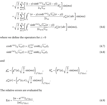
The relative errors are evaluated by

Err =u–u γ(α)

L2_(0,π)

u_L2_(0,π)

. (4.9)

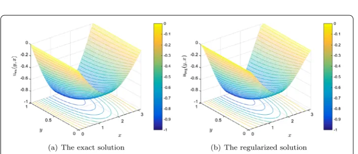
Here, we present graphs illustrating the numerical example, which we are considering. Table1shows that the smallerα, the smaller the error between the exact solution and the regularized solution, and the errors are acceptable. Specifically, in Fig.1, we can see the evaluation results aty= 0.1 andy= 0.3. Moreover, we also show 3D graphs of the exact and regularized solutions throughout the domain (0, 1)×(0,π) in Fig.2. Seen from that point of view, the result of the method of correction is effective.

5 Conclusions

Problem (1.1) was solved using two regularization methods based on problems (3.1) and (3.2). Convergence and stability estimates, as the noise level tends to zero, are formu-lated and proved. Numerical examples support the theoretical findings of the paper. In future work we hope to consider extending the current study to nonlinear sources to allow for an even wider range of physical applications in for example nonlinear elastic-ity.

Table 1 The errors between the exact solution and the regularized solution aty= 0.1 andy= 0.3 for

α∈ {0.1; 0.01; 0.001}

Errors α= 10–1 _{α= 10}–2 _{α= 10}–3

Err(y= 0.1) 0.0575122776 0.0335725277 0.0267921267

Figure 1The exact and regularized solutions aty= 0.1 (a) andy= 0.3 (b) forα∈ {10–1_{, 10}–2_{, 10}–3_}

Figure 23D graphs of the exact and regularized solutions

Acknowledgements

Not applicable.

Funding

Not applicable.

Availability of data and materials

Not applicable.

Competing interests

The authors declare that they have no competing interest.

Authors’ contributions

The authors declare that the study was realized in collaboration with the same responsibility. All authors read and approved the final manuscript.

Author details

1_{Department of Research Management, Thu Dau Mot University, Binh Duong, Vietnam.}2_{Department of Mathematics}

and Computer Science, VNUHCM—University of Science, HoChiMinh City, Vietnam. 3_{School of Mathematics, Statistics}

and Applied Mathematics, National University of Ireland, Galway, Ireland. 4_{Faculty of General Sciences, Can Tho University}

of Technology, Can Tho City, Viet Nam.5_{Institute of Research and Development, Duy Tan University, Da Nang, Vietnam.} 6_{Applied Analysis Research Group, Faculty of Mathematics and Statistics, Ton Duc Thang University, Ho Chi Minh City,}

Vietnam.

Publisher’s Note

Springer Nature remains neutral with regard to jurisdictional claims in published maps and institutional affiliations.

References

1. Antman, S.: Nonlinear Problems of Elasticity, 2nd edn. Applied Mathematical Sciences, vol. 107. Springer, New York (2005)

2. Berchio, E., Gazzola, F., Mitidieri, E.: Positivity preserving property for a class of biharmonic elliptic problems. J. Differ. Equ.229, 1–23 (2006)

3. Berchio, E., Gazzola, F., Weth, T.: Critical growth biharmonic elliptic problems under Steklov type boundary conditions. Adv. Differ. Equ.12, 381–406 (2007)

4. Chang, A.S.Y.: Conformal invariants and partial differential equations. Bull. Am. Math. Soc.42, 365–393 (2005) 5. Ciarlet, P.: Mathematical Elasticity. Studies in Mathematics and Its Applications, vol. 27. North-Holland, Amsterdam

(1997)

6. Courant, R., Friedrichs, K., Lewy, H.: Über die partiellen Differenzengleichungen der mathematischen Physik. Math. Ann.100(1), 32–74 (1928)

7. Gazzola, F.: On the moments of solutions to linear parabolic equations involving the biharmonic operator. Discrete Contin. Dyn. Syst.33, 3583–3597 (2013)

8. Gazzola, F., Grunau, H.C., Sweers, G.: Polyharmonic Boundary Value Problems: A Monograph on Positivity Preserving and Nonlinear Higher Order Elliptic Equations in Bounded Domains. Springer, Berlin (2010)

9. Kal’menov, T., Iskakova, U.: On a boundary value problem for the biharmonic equation. In: AIP Conf. Proc., vol. 1676 (2015)

10. Kal’menov, T., Iskakova, U.: On an ill-posed problem for a biharmonic equation. Filomat31(4), 1051–1056 (2017) 11. Meleshko, V.V.: Selected topics in the history of the two-dimensional biharmonic problem. Appl. Mech. Rev.56,

33–85 (2003)

12. Nair, M.T., Pereverzev, S.V., Tautenhahn, U.: Regularization in Hilbert scales under general smoothing conditions. Inverse Probl.21(6), 1851–1869 (2005)

13. Nguyen, H.T., Kirane, M., Quoc, N.D.H., Vo, V.A.: Approximation of an inverse initial problem for a biparabolic equation. Mediterr. J. Math.15, 18 (2018)

14. Sweers, G.: A survey on boundary conditions for the biharmonic. Complex Var. Elliptic Equ.54, 79–93 (2009) 15. Tuan, N.H., Lesnic, D., Viet, T.Q., Au, V.V.: Regularization of the semilinear sideways heat equation. IMA J. Appl. Math.,

84(2), 258–291 (2019)

16. Tuan, N.H., Quan, P.H.: Some extended results on a nonlinear ill-posed heat equation and remarks on a general case of nonlinear terms. Nonlinear Anal., Real World Appl.12(6), 2973–2984 (2011)

17. Tuan, N.H., Thang, L.D., Khoa, V.A.: A modified integral equation method of the nonlinear elliptic equation with globally and locally Lipschitz source. Appl. Math. Comput.265, 245–265 (2015)

18. Tuan, N.H., Thang, L.D., Khoa, V.A., Tran, T.: On an inverse boundary value problem of a nonlinear elliptic equation in three dimensions. J. Math. Anal. Appl.426, 1232–1261 (2015)