R E S E A R C H
Open Access
Efficient link scheduling for rechargeable
wireless ad hoc and sensor networks
Guodong Sun
1, Guofu Qiao
2*and Lin Zhao
1Abstract
We study the link scheduling for rechargeable wireless ad hoc and sensor networks to improve network throughput. Efficient link scheduling is highly critical for wireless networks, and a lot of efforts have been made to address this issue. The previous work which only considers how to reduce interference within close-by links, however, fails to improve the network throughput for rechargeable wireless network in which a node, powered by ambient energy (such like solar and vibration) has to be recharged before it can communicate with other nodes. Thus, link scheduling with rechargeable nodes is constrained not only by co-channel interference but also by energy replenishment of the node. In this paper, we develop efficient link scheduling algorithms to improve the network throughput of
rechargeable wireless ad hoc and sensor networks. The proposed design, based on realistic network models and mathematical formulation, achieves constant ratio of the best solution. Besides the theoretical analysis, simulation experiments are conducted to evaluate our algorithms.
Introduction
Many wireless network applications, such as sensor net-works and wireless ad hoc netnet-works, are expected to operate a long time with limited energy source. Harvest-ing the environmental energy to power wireless nodes is a promising method to address the conflict between node’s limited energy and application lifetime require-ments. For example, the renewable energy transformed from solar, vibration, thermo, water flow, and corrosion can be employed to recharge wireless nodes [1-6]. How-ever, two major characteristics of rechargeable wireless network make it more difficult to optimize communi-cation performances, in comparison with the traditional wireless network without depending on renewable energy. First, the operation of rechargeable node often has to be intermittent. In practice, the energy-harvesting rate is usually lower than the energy consumption rate. For example, the energy generated by mechanical vibration is about the level 300μW/cm2[2], that is, a vibration energy harvester with a surface of 40 cm2 can output 12 mW of energy. If such harvester powers Micaz mote working with 60 mW of energy, a recharging cycle of at least 5 s is
*Correspondence: [email protected]
2School of Civil Engineering, Harbin Institute of Technology, 77 Huanghe Rd, Harbin 150006, China
Full list of author information is available at the end of the article
needed before a 1-s task can be carried out. For the ther-moelectric energy harvester fitted on a wristwatch of body health care sensor network [5], it outputs energy at the level of 22μW, and then it needs a longer recharging dura-tion. Hence, a node has to wait until it accumulates suf-ficient energy before it can perform tasks of computation and communication. For applications demanding some degree of real-time , therefore, the network throughput would deteriorate significantly without link scheduling.
Second, the ability of harvesting energy is usually het-erogeneous among distinct nodes. This is because the producing ability of environments and the energy-accumulating ability of harvesters are possibly different. For instance, in a vibration-powered scenario, a harvester with a small surface of sensing vibration signals will out-put power lower than that outout-put by the harvester with a large sensing surface, and then it may need more time for recharging before communication can be carried out. Thus, a new challenge facing the link scheduling is that the heterogeneity of ambient power sources must be accounted for.
In this paper, we focus on the link scheduling prob-lem for a rechargeable wireless network to improve the network throughput. Even though link scheduling has attracted a lot of attention in recent years [7-16], the previous works, which only consider how to avoid the co-channel interference in throughput improvement, often
gives undesirable or even failed answers in the case with energy replenishment. These previous link scheduling policies have shown their efficiency in network through-put and energy consumption. However, we argue that these polices are all based on a precondition: the two end-nodes of each link is available in terms of energy whenever it is to be scheduled. But this precondition cannot always be satisfied in many energy-rechargeable wireless networks, especially scenarios with extremely low energy-harvesting rate (such as applications powered by vibration, corrosion, or thermo energy).
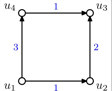
For a simple four-node network operating under suc-cessive, synchronized time slots, Figures 1 and 2 show two link schedules with and without considering energy replenishment, respectively. Suppose here that links (u2,u3)and(u1,u4)of Figures 1 and 2 interfere with each other. Figure 1 shows a schedule using three distinct time slots for all four links. Figure 2 considers the restriction posed by both interference and energy replenishment, and assumes that each node needs some time units to recharge its energy buffer. For simplicity, we assume that the energy buffer of each node contains only energy that transmits or receives a single packet. If a node recharges fully at time slot t, it can then communicate at t + 1. If the energy buffers of all four nodes of Figure 2 are empty at time 0, link (u1,u2) can just be scheduled after time 6, even thoughu1will have already recharged fully at time 2. Sim-ilarly, due to the restriction of energy replenishment, we complete scheduling all four links of Figure 2 until time 12. Therefore, we can see that the couple of interference and energy replenishment determines the link scheduling and its performance. Moreover, it is worth pointing out that the total schedule time in Figure 2 should not be measured
Figure 1A link schedule with only interference restriction.In this case, links(u2,u3)and(u1,u4)interfere with each other, and the blue number represents the assigned time slot.
Figure 2A link schedule with restrictions of interference and energy replenishment.In this case, links(u2,u3)and(u1,u4) interfere with each other, and the blue number represents the assigned time slot. Here,ui|xmeans thatuineedsxtime slots to harvest the energy enough to transmit/receive a single packet.
by the number of time assignments for all links, as done in Figure 1, but by the span of time units for all links. This is an important difference from the previous wireless link scheduling without energy replenishment or from the frequency assignment for cellular network.
The main objective of our work is to find a link scheduling for a rechargeable wireless network, using a period as small as possible, while guaranteeing that each node has enough energy when being scheduled. To effi-ciently address the link scheduling restricted by both energy harvesting and co-channel interference, we employ the following studies. First, we take the link schedul-ing problem under a more realistic network model, the request-to-send (RTS)/clear-to-send (CTS) model, under which the communication graph can be an arbitrary geo-metric graph. We also use a practical energy-harvesting model, which profiles a large class of ambient energy sources outputting very low energy, such as vibration, thermo, and corrosion. Based on these realistic models, we transform the link scheduling problem to a vertex-coloring problem, using the concept of conflict graph which profile interferences in a co-channel wireless net-work. Second, we design two effective, low-complexity algorithms for link scheduling in two cases - with and without considering traffic flows. Specially, we provide theoretical bounds for our algorithms in these two cases. Finally, we evaluate our algorithms via primary simulation experiments.
Related work
from its surroundings. More effort is put on the design of energy-recharging circuit which can be integrated to customer-off-the-shelf sensor mote, such like Crossbow Mica-family mote and Berkeley Telos mote. The early work is attributed to Kansal et al. [1] who design a solar-powered sensor node and an energy metric, EEHF, which assigns more loads at nodes with a higher energy-harvesting rate. Helimote [17] is an energy-energy-harvesting system with a single storage for solar energy. Built on Mica2 mote, Helimote recharges two AA Ni-MH batter-ies. Helimote can learn its energy availability and usage via an energy monitoring component. Jiang et al. [18] design Prometheus, a hybrid energy storage system for solar energy. Built on Telos, Prometheus mote is pow-ered by the supercapacitors, called the primary energy buffer, or by the rechargeable Li-ion battery, called the sec-ondary energy buffer. If the primary buffer energy is less than some threshold, the mote falls back to the secondary buffer until the primary one recharges fully again. Similar to Prometheus, AmbiMax [19] uses hybrid energy storage, but AmbiMax tracks the maximum power point automat-ically, without needing the control of MCU. EverLast [20] is a supercapacitor-driven sensor mote, and it uses PFM controller and regulator to harvest the solar energy. To track the maximum power point, EverLast is built with a complex charging circuit. Qiao et al. [21] discuss the fea-sibility of powering wireless nodes with the energy from corrosion process.
Besides the platform designs, there are recently some studies focusing on the routing algorithms in recharge-able wireless network. Lin et al. [22] developed a routing scheme to optimize the network throughput by an energy model assuming heterogeneous energy-harvesting rates. CHESS [23] is a routing metric for energy-harvesting sen-sor networks. It uses hybrid energy storage and assigns different costs to the energy in supercapacitor and the rechargeable batteries and favors routes with more energy. Eu et al. [24] studied optimal routing in an energy-harvesting sensor network with optimal relay node place-ment and investigated the impact of routing and node placement on the network performance. In [25], they proposed a lexicographically maximal data rate assign-ment for each source node such that no node runs out of energy. In [26], two schemes, QuickFix and SnapIt, were proposed. QuickFix computes the static routes using the sub-gradient method, and based on QuickFix, SnapIt adaptively allocates sampling rate for a single node with a possibly dynamic recharging rate. In [27], the authors investigated the finite-horizon problem in rechargeable sensor networks and proposed an approach including three steps: first, optimize the throughput of a single node; second, design an online algorithm, assuming that the future energy-harvesting rate is predictable; and third, to improve complexity, propose a heuristic distributed
algorithm which is optimal with homogeneous energy-harvesting rate of nodes.
As a kind of resource allocation to optimize network throughput, link scheduling has been studied extensively in the past few years. Essentially, link scheduling can be reduced to graph coloring problems. An early work [28] has a vertex color graph Gwith δ + 1 colors, where δ is the minimum degree in G. A unified framework for TDMA-, FDMA-, and CDMA-based multi-hop wireless network is proposed in [29], in which the time slot assign-ment for all edges is at mostO(θ )times the best solution, whereθevaluates the degree that the graph can be decom-posed. In [30], aO(+1)-coloring is designed with time
O(logn+), whereis the maximum degree ofG. How-ever, those algorithms do not consider the interference of practical wireless application and then cannot work directly in wireless networks.
Gandham et al. [13] designed a two-phase approach which first computes a valid edge coloring and then assigns directions for all edges to avoid interference. The performance is guaranteed only with tree topology. The coloring in [31] is a O(logn) distributed algo-rithm usingcolors, but in the unit disk graph (UDG) model, they may make interfering links still use the same color. Kodialam et al. [32] considered jointly rout-ing and link schedulrout-ing with the protocol interference model and solved the scheduling problem as an edge-coloring problem. They also extended the algorithm to the multi-radio and multi-channel scenario [33]. Alicherry et al. [9] established necessary and sufficient conditions for interference-free link schedule and proposed a simple greedy algorithm based on the UDG model. Sharma et al. [34] defined aK-hop interference model under which no two links withinKhops can be scheduled simultaneously and presented a centralized greedy matching algorithm with a constant factor. The same authors studied greedy maximal scheduling with the K-hop interference model [35]. Wan et al. [36] studied the link scheduling with a physical interference model.They also presented a link scheduling algorithm without requiring node’s location information [15]. Koulali et al. [37] designed a centralized power control scheme for rechargeable wireless multime-dia sensor networks.
Models and assumptions
In this section, we will present the wireless communica-tion models and some assumpcommunica-tions used in our study and will describe the link scheduling problem formally.
Network and interference models
Figure 3The primary and secondary interferences in link scheduling.
communication graphG=(V,E), whereEis the set of all radio links among nodes. Denote link(vi,vj) byi,j. The
transmission range of each nodeviofV isri. It is neces-sary for nodevjto correctly receive data fromvithat the Euclidean distance betweenviandvj,||vi−vj||, is not larger thanri. Note here that||vi−vj|| ≤riis not the sufficient condition for(vi,vj) ∈ Ebecause some links may be cut
off by obstacles or forbidden by topology controls as well as routing policies. Each nodevihas an interference range,
which is generally equal to or greater thanri. For the ease
of analysis, the interference range is hereafter assumed to be the same as the transmission range. But we use a more realistic interference radius setting in simulation experi-ments. We assume that the operation time of all nodes is equally slotted and synchronized and that the size of all packets are the same. In general, the link scheduling is to assign every link a set of time slots. Letτ denote the time span of a slot and assume that in a slot, a node can either
transmit or receive only one packet, except for necessary control bits.
In a single-radio network, interference between adja-cent or close-by links has to be avoided in order to reduce the delay or save energy. There are two major kinds of interferences: primary interference and secondary inter-ference. When a node transmits and receives at the same time slot, primary interference happens; when a node receive two or more distinct transmissions, secondary interference occurs. In Figure 3, links p,q andq,p can-not be scheduled concurrently for a single-radio network. Additionally, since node uq locates within the
interfer-ence range of vi, links i,j and p,q cannot be scheduled
at the same time to avoid conflict at vj. Besides, in real scenarios, for improving the network reliability or other network performance, there are other kinds of interfer-ence that pose restrictions on link scheduling, such as the RTS and CTS control schemes used in 802.11-like MAC protocols.
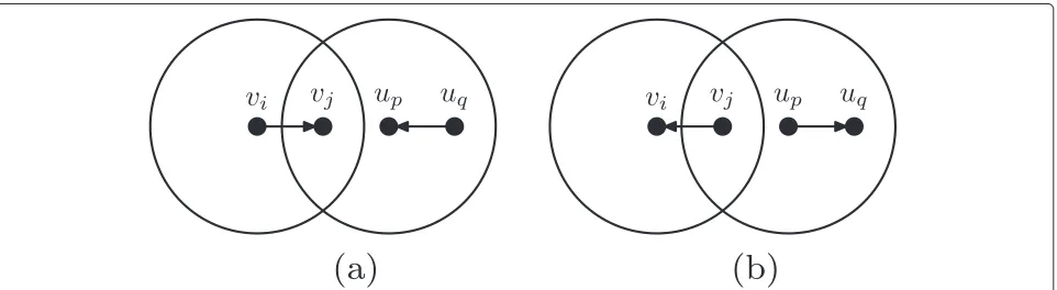
In this study, we use the RTS/CTS-based interfer-ence model [9,38-40], which is more realistic than the UDG model extensively used in previous literature. Under RTS/CTS model, all nodes within the interference range of either a transmitter or a receiver are not allowed to communicate. In detail, if two links i,j andp,q can be active simultaneously, it must be satisfied that vi,vj,vp,
and vq are four distinct nodes, and vi as well as vj is
not covered by the interference regions of vp and vq,
and vice versa. In Figure 4a, the RTS message from vj
will be listened by up, so up must postpone its trans-mission to uq. In Figure 4b, if vj admits to receive data from vi, vj will send a CTS message, which will also be received byup, thenp,qshould not be scheduled while
i,jis active. Clearly, in comparison with the UDG model,
the RTS/CTS model neither requires that all nodes have the same radio range nor assumes that two nodes within each other’s radio range must be able to communicate. Therefore, the RTS/CTS model does not preclude the
topology or transmit power control algorithms, thereby being more realistic and layer-independent for real scenarios.
Energy harvesting model
In practice, the rechargeable wireless node is equipped with a harvester unit which transforms ambient signals into trickles of electrical energy. The energy buffer of the rechargeable node is often very limited in capacity due to the constraints of package size and cost. In addi-tion, for some scenarios where the environmental energy is extremely low in output power, nodes have to use longer periods of time to recharge their energy buffer before they can carry out tasks. Therefore, it is often impossible for a node to quickly buffer much energy for longtime, continual operation. Combined with the chal-lenge of co-channel interference, the constrained and intermittent energy provision motivates us to investi-gate efficient link scheduling in the context of recharg-ing wireless networks, such that the network throughput can be improved by carefully assigning time slots for links.
For simplicity, we only consider the energy consump-tion in communicaconsump-tion because in low-rate, low-power wireless scenarios, communication consumes significant energy in comparison with computation. We also assume that transmitting and receiving data consumes identi-cal power, e.g., for TI’s CC2420 radio chip, the current consumption in transmitting and receiving are 17.4 and 19.4 mA, respectively.
Denote bythe energy consumed by one-packet trans-mission or reception. In data communication with acknowledgement (ACK) scheme, represents the total energy used in transmitting a packet and receiving the ACK message. In the real world, the surrounding energy distributes unevenly because of different natural envi-ronments or deployments. Therefore, different nodes may have different energy-harvesting abilities - differ-ent recharging durations. Letγ be the duration (in time slot) for a node to harvest 1 energy, and obviously, γ evaluates the energy-harvesting ability of that node. If γ = 0 for a node, then it means that this node has an always-available energy source. We assume that for a given node, its energy-harvesting duration is constant or varies in a very small range and is knowna priori. This assumption profiles many typical environmental energy sources in practice, such as the vibration in factory [2], the thermo-heat of the human body in mobile health care [5], and the corrosion of steel-concrete structures [3], where all the energy generation rates vary little even in a long period, say, several weeks, or even months. In this paper, the rechargeable nodes work with two alternate states: active and dormant states [41-44]. In detail, when a node has enough energy, it will enter the active state to
perform computation and communication; otherwise, it will enter the sleeping state while leaving only the harvest-ing module active.
Problem formulation
In a time-slotted wireless network, a link schedule is to find a time slot assignment for each link, and it is called
validif at any time slot, two active links are not conflict-ing.Tis called theschedule periodif it takesTtime slots to schedule all the links once (without considering traf-fic load) or all the flows once (with considering traftraf-fic load). Link scheduling often aims at improving the net-work throughput, i.e., reducingTto be as small as possible while making the network conflict-free.
Besides the interference restriction, the link schedul-ing in rechargeable wireless network is restricted by the energy dynamics of node because one or two end nodes of a link may need more time to recharge until it (they) harvest sufficient energy to transmit or receive a packet. In this paper, therefore, the objective of link scheduling is to determine a time slot assignment for all links or flows with a smallest possible schedule period, such that not only interference can be avoided, but also each node has enough energy upon being scheduled.
For a given communication network, the link schedule is essentially a kind of edge-coloring problem in the commu-nication graph. Different from the UDG model, however, our RTS/CTS model leads to a more realistic but more complex interference relationship among close-by links. To address this problem, we use the concept of the con-flict graph [10,11,40] to transform link scheduling to a vertex-coloring problem as follows.
LetFGbe the conflict graph of a given communication graphG. Each edge (link) ofGis converted to a vertex of
FG, and two vertices ofFG (both of them represent two
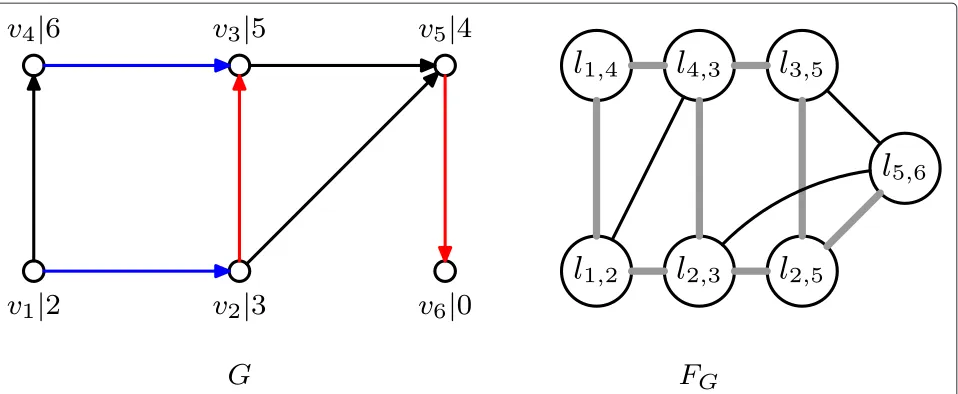
links of G) are connected with an edge if they conflict with each other inG, according to the RTS/CTS model. Figure 5, for example, shows communication graphGand its conflict graph FG. It is clear that we can obtain an
interference-free link schedule forGby finding a proper vertex-coloring of FG. To make the conflict graph able
to evaluate the level and dynamics of the node’s energy, we extend the above conflict graph model by adding a weight, denoted by i,j, for each vertex ofFG, where i,j=
max{wi,wj}andwi andwjrepresent the earliest possible time forviandvjto be scheduled, respectively. Obviously,
wivaries according to time and then is determined byγi,
the harvesting duration ofvi, and by the current schedule
Figure 5Converting a communication graphGto a conflict graphFG.InG,1,2interferes with4,3, and2,3interferes with5,6. InFG, the thick gray edge and the thin dark edge describe the primary interference and secondary interference, respectively.
Note that in the context of rechargeable wireless net-work, the concern on vertex-coloringFGis not to achieve the smallest possible number of colors (time slots), much the way the previous link scheduling schemes assuming always-available energy source does, but to find a sched-ule for all links with the smallest possible span of time slots, which is the way to evaluate and improve the perfor-mance of link scheduling for energy-rechargeable wireless applications.
Algorithm design
In this section we will, in detail, present two link schedul-ing algorithms for rechargeable wireless network, with and without considering the traffic load, and theoretically analyze their complexity and prove their performance.
Scheduling without traffic load
We first introduce some necessary definitions and proper-ties before presenting a centralized link scheduling algo-rithm and proving its performance. For each vertexuof
G, besides its harvesting durationγu as well as its earli-est schedulable timewi, we also use two other variables
to describeu’s state at timet:euandsu, whereeu
repre-sents the energy level ofuandsuthe times thatuhas been
already scheduled till timet. At a given timet, if we know γuandsu, then we can calculate the current energy level
ofuby Equation 1. At timet, ifeu > 1,ucan be
sched-uled immediately, that is,wu= t, and ifeu= 1, we have wu=t+1. Ifeu< at timet, however,uneeds more time
to collect sufficient energy before it can be scheduled, and
wucan be calculated by Equation 2:
eu=
t γu−
su× (1)
wu=t+γu(−eu)+1 (2)
According to the calculation ofwuof each vertexu, we can easily determine the earliest schedulable time of a link. For two vertices (links)i,jandp,qofFG, if i,jis less than p,qor if i,j= p,qbut the degree ofi,jis less than that
ofp,q, we say that linki,jproceedslinkp,q.
Among the centralized link scheduling algorithms pre-viously presented, the common method is to use the greedy graph coloring to assign each vertex the minimum possible time slot. There is a critical difference among these works: they use different orders to greedily color vertices. Our centralized scheduling is also based on the greedy vertex coloring used in general graphs: the earli-est available vertex ofFGwill always be first colored with
the smallest possible time slot (color), and of two links with identical earliest available time, the link with mini-mum degree will be scheduled preferentially. Algorithm 1 details the centralized link scheduling without consider-ing traffic load. Construction of conflict graph needs time ofO(m2), wheremis the number of links ofG. It can be easily deduced that in Algorithm 1, every vertex ofFGis
selected only once and that all unselected vertices adja-cent to the currently selected vertex are scanned to update their earliest schedulable times. So the time complexity of Algorithm 1 is also O(m2). Next, we will prove the performance of Algorithm 1.
Let Rx be the interference region of vertexx, a circle
centering x and with radius ofrx. LetNx be the set of
vertices whose interference radius is at leastrx and who
interfere with some vertices covered byRx. The
interfer-ence radius of a link u,v is defined asru,v (orr) which equals max{ru,rv}. And denote byI()the set of links
Algorithm 1Link scheduling without traffic load
Require: G, the communication graph
Ensure: a valid link schedule for all links ofG
1: For each vertexuofG, seteu =0,su =0, andwu =
γu+1. ConstructG’s conflict graph,FG, and letFG = FG.
2: whileFG is not emptydo
3: Find vertexu,vofFG such that it proceeds all other
vertices.
4: If none ofu,v’s neighbors inFGis already assigned
to time slot u,v, then assign time slot u,vtou,v;
otherwise, assignu,v the minimum possible time slot not yet used by any of its neighbors of FG.
Denote bykthe time slot foru,v.
5: Increasesuandsvboth by one. Update the energy level of u by Equation 1. If eu ≥ , then wu is set to bek+1; otherwise, it is set to be the time slot calculated by Equation 2. Similarly,evandwv
can be updated also. Notice that updating wu or wvchanges consequently the weights of other links
incident withuorv. Delete vertexu,vfromFG.
6: end while
Theorem 1. Given a vertex vx and any subset Vx of Nx,
there exists a vertex subset Vxof Vxwith size at least|Vx|/ϕ such that each vertex of Vxinterferes with or is interfered by at least one other vertices, whereϕis upper-bounded by 30.
Proof.See Appendix.
Theorem 1 implicates that inNx, a set of vertices that
possibly interferes with the transmission fromvxor tovx,
there exists a subset ofNx, in which for any two vertices, ui anduj, ui interferes withuj, uj interferes withui, or
both. Even though Theorem 1 estimates only the degree of local interference at level of vertex, we can extend it to the level of link using Corollary 1.
Corollary 1. For any given link, there exists a subset of
|I()|of size at least|I()|/2ϕ, in which any pair of links interferes with each other under the RTS/CTS model.
Proof.See Appendix.
In fact, Corollary 1 indicates that if a vertex (link) 0 of conflict graph FG has k neighboring vertices (links),
1,2,. . . k, then0 must have at leastk/2ϕ neighbors that are mutually interfering; in other words, the graph formed by thesek vertices and the edges between them contains a clique of orderk/2ϕ.
Theorem 2. For a given communication graph G, if its
conflict graph is a clique of order m, denoted by FGK, then
we need as least (γmin+m+1) time slots for scheduling all links, whereγminis the shortest harvesting duration of G’s vertices and m is the number of links of G.
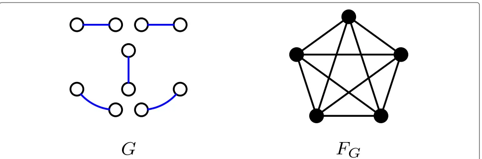
Proof.This theorem can be proven by first considering an extreme case, in which for any two vertices (links) of
FGK, they are not incident on any vertex ofG. As shown in Figure 6, for example, all five links inGare interfering and form cliqueFGKof order five, but they have no com-mon vertices. In such a case, the energy levels at both end vertices of a given link put no effect on scheduling other links ofGin terms of the energy restriction. The sched-ule period depends only on close-by interferences and the local harvesting rates. Suppose that the fastest possible schedule isTK time slots in this case; obviously,TK is at least (γmin+m+1).
If two links ofGis incident in Figure 6, the conflict graph is still cliqueFGK; however, coloring these two adjacent ver-tices (links) ofFGKwill have to be affected (restricted) by the energy replenishment of the incident vertex. Thus, the schedule period must be greater than or equal toTK =
γmin+m+1, wheremis the order of the conflict graph.
Because what we are concerned about is the span of time slots for all links, it is reasonable to treat the maximum assigned time slot as the schedule period. Theorem 2 helps in determining an effective lower bound for an arbitrary wireless network with constraints of co-channel interfer-ence and energy replenishment. Based on Theorem 2, the following theorem will prove that Algorithm 1 can achieve a constant factor of the optimal link scheduling.
Theorem 3. Algorithm 1 computes a valid time slot
assignment using at most2ϕ(γmax+1)times the time slots needed by the optimal schedule, whereγmaxis the longest harvesting duration of vertex in G andϕis the upper bound deduced in Theorem 1.
Proof.Note that in step four of this algorithm, we always assign a vertex which is the time slot that has not yet been used by any of its adjacent vertices ofFG. Thus, it is easy
to know that Algorithm 1 is conflict-free. Next, we prove the algorithm’s performance.
LetToptandTAlg1be the scheduling period’s output by the optimal algorithm and Algorithm 1, respectively. Sup-pose thatvis the vertex with the maximum degree inFG
and its degree is denoted byδv. Corollary 1 implies that forv, there exists a clique (includingvand its neighbors), whose size is at least(δv +1)/2ϕ. Then, by Theorem 2, we need at least(γmin+(δv+1)/2ϕ+1)time slots for scheduling all vertices (links) of the clique, without con-sidering other vertices ofFG. So we have an effective lower bound for the optimal algorithm’s performance, that is,
Figure 6Illustration for the proof of Theorem 2.InGwhose conflict graphFK
Gis of form clique, all links interfere mutually but are not incident with one another.
It is not straightforward to derive a tight upper bound of TAlg1. Here, we use some theories about T-coloring problem [45-47] for the proof. We construct aT -coloring-based schedule for G, whose period is longer than that of Algorithm 1 but is easy to be upper-bounded. Given a graph, aT-coloring is to assign each vertex an integer such that the absolute value of the difference between integers for adjacent vertices does not belong toT which is called
T set. In our scenario, for example, if the T set is {0, 4} and a vertex ofFG is the given color (time slot) c, then
its neighbor (links) can be given neither colorcnor color
c+4.
Now let T set be {0, 1, 2,. . .,γmax}. In the schedule based on thisT set, any two adjacent vertices (links) of
FG are sure to be conflict-free because 0 ∈ T, mean-ing that two adjacent vertices will not be assigned the same time slot. In fact, for any two adjacent vertices of
FG, the difference of time slot assigned to them is at least γmax + 1, which is according to the definition of the T set, and therefore, such a T set results in a T -coloring schedule that is feasible for rechargeable wireless network, in terms of interference and energy. It is clear that the T-coloring-based link scheduling always waits at least (γmax + 1) time slots between two consecutive schedules of two interfering links, without considering whether or not the second link is already available before being scheduled. In contrast, Algorithm 1, based on the maximal scheduling policy, always schedules a link the moment it is feasible in terms of both energy and inter-ference and consequently uses less time than the above
T-coloring counterpart does. Obviously, the performance ofT-coloring-based scheduling provides a natural upper bound for Algorithm 1.
It is given in [45,46] thatT-coloring graphG, the mini-mum span over allT-colors forG, denoted by spT(G), can be expressed by(r+1)(χ (G)−1), whereχ (G)is the chro-matic number ofG(without being restricted by theTset)
andris the maximum integer of theTset. Recall that we have assumed that the maximum degree of FG isδv; we
know that the chromatic numberχ (FG)must be less than or equal to(δv+1), according to the principle of graph
theory. Furthermore, we have spT(G) ≤rδv. Thus,
Algo-rithm 1 uses at most(γmax+1)δvtime slots for scheduling
all links once, that is,TAlg1≤(γmax+1)δv:
TAlg1
Topt ≤
(γmax+1)δv
γmin+1+(δv+1)/2ϕ
(3)
< (γmax+1)(δv+1) (δv+1)/2ϕ = 2ϕ(γmax+1)
According to the lower bound for Topt and the upper bound forTAlg1, we have Equation 3, that is, the schedule period of Algorithm 1 is at most 2ϕ(γmax+1)times that of the optimal solution.
Note that in the proof of Theorem 3, we assume that the vertex with the maximum degree inFGhas the worst
harvesting duration. Thus, the upper bound for the per-formance of Algorithm 1 can be improved with a tighter analysis if we have further knowledge about the distribu-tion of harvesting rates among nodes.
Scheduling with traffic load
The algorithm proposed above is based on the assumption that all links are needed to deliver equal traffic load. But not all communication patterns support this assumption, especially the many-to-one wireless sensor networking that uses a few links to collect data from all source nodes. In this section, we will design a more general scheduling framework considering traffic load of link and prove its performance based on the previous analysis.
flows from si to ti that are determined by some rout-ing algorithm. For each link of G, its traffic load can be measured by fi(), wherefi()means the ith flow
traversing through link. Exactly, if the bandwidth of isb, thenneeds to be assignedb1
fi()time slots
in a single schedule of all flows, which is the link traf-fic load ofin terms of time slot. In practice, the traffic load through each link can be determined once the rout-ing algorithm terminates correctly, and in general, a link is possibly scheduled multiple times - assigned with multiple time slots - for scheduling all flows.
Algorithm 2Link scheduling with traffic load
Require: G, the communication graph, and the traffic
loadρof each link
Ensure: a valid link schedule for all flows ofG
1: Construct G’s conflict graph, FG. As shown in
Figure 7, add vertices and edges toFG, according to the following steps (from 2 to 4).
2: Declare an empty graphFG
3: For a given vertex (link)ofFG, ifρ>0, then we add toFG withρidentical vertices,1,2. . .,ρ, and with the edges connectingiandjofFG (1≤i<j≤ρ). 4: For any two adjacent vertices1and2ofFG, add to
FG the edges connectingi1andj2, where 1≤i ≤ρ1 and 1≤j≤ρ2.
5: Run steps 2 to 6 of Algorithm 1 directly onFG, which
outputs a time slot for eachjiofFG.
6: Assign linkofGall the time slots used byi(1≤i≤
ρ)ofFG.
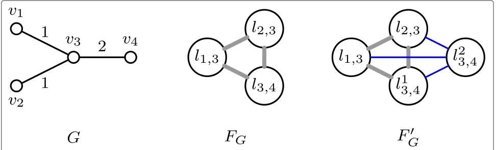
To schedule all flows, Algorithm 2 is proposed to assign each link one or more time slots according to the link load. The basic idea of Algorithm 2 is to extend the conflict graph used by Algorithm 1, such that the vertex needing multiple schedules are decomposed to equal-quantity ver-tices, each of which only needs to be scheduled once using Algorithm 1. Figure 7 shows a walk-through example. The
communication graphGwill deliver two flows: one is from
v1to v4 and the other is fromv2to v4. Both flows tra-verse pastv3, so link1,3takes the load of one unit,2,3 takes the load of one unit, and3,4takes the load of two units. The middle graph in Figure 7, FG, is the conflict
graph ofGwithout considering the traffic load. To sched-ule two flows, however, we need to assign three links1,3, 2,3, and3,4: one time slot, one time slot, and two time slots, respectively. We rename3,4using13,4and add into
FGa new vertex, denoted by23,4, such that23,4relates with other vertices as3,4does. In other words, we connect23,4 andif there is an edge between13,4andinFG. Of course
we should also add an edge between13,4and23,4. In doing so, the conflict graphFGis extended toFG, shown on the
right side of Figure 7. Clearly,FG not only demonstrates the restriction of interference in link scheduling, as FG
does, but also indicates the number of times for schedul-ing each link. Now we can complete schedulschedul-ing all flows ofGas soon as each vertex (link) ofFG is scheduled once. From the process of extendingFG intoFG, we can see
that the complexity of such extension depends on flows over communication networkG, i.e., on the weight (traf-fic load) of each link. For a wireless network withnnodes, the traffic load through any node is of orderO(n). Step 3 of Algorithm 2 examines each vertex to verify whether its weight is greater than one, consumingO(m)time wherem
is the number of vertices ofFG(or the number of links of G). Combining steps 3 and 4 of Algorithm 2, the extension fromFG toFG requiresO(mn)time. Since the
construc-tion of FG is of time complexityO(m2), as analyzed in
the previous section, Algorithm 2 terminates with time of orderO(max{m2,mn}). We next prove the validity and performance of Algorithm 2 via Theorem 4.
Theorem 4. For a given communication graph,
Algo-rithm 2 returns a valid link schedule for all flows, which uses at most k times that of the optimal solution consider-ing the traffic load if Algorithm 1 uses at most k times the optimal solution without considering the traffic load.
Proof. For a given communication graphGand a set of flows throughG, suppose that the traffic load of each link ofGis at least one. LetTOPTf be the minimum span of time slots for scheduling all vertices ofFG, considering link traf-fic, and letTOPTbe the minimum span of time slots for scheduling all vertices ofFG, without considering link traf-fic. IfTOPTf >TOPT, then we can use the optimal schedule onFG to construct a new schedule forFG with a smaller
period. SoTOPTf is not the best solution; it contradicts. Similarly, we know thatTOPTf < TOPTis impossible too. Thus, we haveTOPTf = TOPTfor a givenGand any flow assignment throughG.
Essentially, the operation of Algorithm 2 is equivalent to running Algorithm 1 on the extended conflict graph,FG. If the schedule period forFG output by Algorithm 1 isk
timesTOPT, then it is alsok timesTOPTf . Note that it is possible for a routing to forbid some links, which makes them not to be scheduled at all; however, this theorem still holds in such a case.
Performance evaluation
In this section, we conduct extensive simulations to eval-uate our algorithms and compare their performance with the lower bound of the optimal solution. In the case with-out traffic flows, the lower bound on the optimum is set to be max{γi·δi} +1, whereδiis the degree of vertexviin the
communicationG, and in the case with flows, the lower bound on the optimum is set to be max{γifi}, wherefi
is the total flows pastvi. Clearly, the smaller the ratio to the
lower bound for optimum, the better is the performance of the proposed algorithms.
In simulation, nodes are randomly deployed in a uni-form way within a 40×40 square. The transmit range of node is randomly selected from 10 to 15 and fixed in sim-ulation. For each node, its interference range is set to be twice its transmit range, much the way the IEEE 802.11 scheme works. The time span of a single time slot,τ, is set to be 500 ms which should be able to cover some control messages (RTS, CTS, and ACK), even though we neglect the control message exchange in our simula-tion. Every node randomly selects an energy-harvesting duration from the integer set of{0, 1,. . .,γmax}. Each sim-ulation result is reported with the average of 100 random deployments.
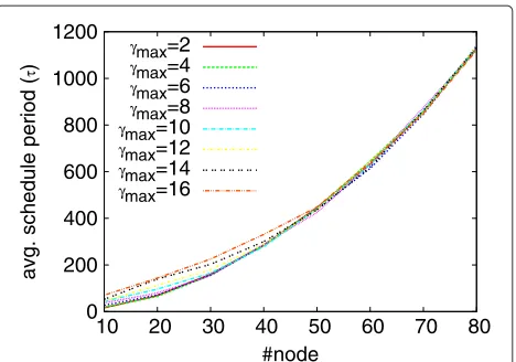
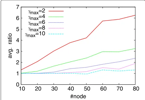
First, we examine the performance of Algorithm 1, which does not consider the link traffic and assumes that each link has the same data arrival rate. Figure 8 shows that given aγmax, when the number of nodes increases, more time is needed as expected. Why does the case with the smallest γmax achieve a schedule period simi-lar to the case with the simi-largest γmax? Figure 9 gives an answer. From Figure 9, we can see that for a network
0
Figure 8The schedule period under the link schedule without traffic flows.
size, the performance of Algorithm 1 becomes better as γmaxincreases. This is because the larger theγmaxis, the larger the deviation of node’s recharging cycles, and then the earliest schedulable times of distinct nodes will not overlap too much, as the case with what the smallerγmax will experience. Additionally, given aγmax, increasing the network size deteriorates the performance due to more interference. Thus, as expected, Algorithm 1 may behave better with less interference, that is, it is more suitable for scenarios with sparse distribution or short radio range.
Second, we evaluate Algorithm 2 which runs with the shortest path routing. Here, the shortest path routing algorithm, using the harvesting ability of nodes as the for-warding metric, always returns a path for each source such that the total harvesting durations of nodes along the path reaches the minimum. Note that Algorithm 2 depends neither on any particular routings nor on the communi-cation patterns (one-to-one, many-to-one, or others). In
0
0
Figure 10The schedule period under the link schedule with traffic flows.
every simulation, we always randomly select 20% nodes as sources, each of which uses a constant rate of one packet/s to report data to the sink node centering the square. Figures 10 and 11 show results that are similar to the case without considering traffic flows, as proven by Theorem 4.
Conclusions
In wireless ad hoc and sensor networks with renewable energy, not only the co-channel interference but also the energy replenishment weighs heavily against increasing the network throughput. So an efficient link scheduling is highly demanded in rechargeable wireless networks, espe-cially in scenarios with very low ability in harvesting ambi-ent energy. To the best of our knowledge, we are the first to investigate how to efficiently schedule links restricted by both interference and energy replenishment. Based on
0
Figure 11The performance ratio under the link schedule with traffic flows.
realistic network models, we first proposed a centralized scheduling for all links without considering the link load, and the achieved period of feasible schedule is within con-stant ratio of the best solution. We then proposed a more general link scheduling algorithm for network flows, with the proven performance of a constant factor. The sim-ulation results also demonstrate the performance of our designs. In this paper, we did not analyze the stability of Algorithm 2 with an arbitrary pattern of network flows. Additionally, it is very difficult and challenging to design a localized link scheduling with a constant factor for a rechargeable wireless network because local decision may dramatically influence future performance in a hard pre-dictable way. In the future, we will focus on these two aspects.
Appendix
Proof of Theorem 1.Given a vertexvxand a subsetVxof
Nx, suppose thatvx’s interference radius and region arerx
andRx, respectively. We divideVxinto three parts,
accord-ing to the locations of its vertices:Vx1whose vertices are withinRx,Vx2whose vertices are out ofRxbut covered by the circle centeringvxand with the radius of√3rx, andVx3
(the other vertices ofVx). In this proof, we only need to prove that for any two verticesuandvofVx, the distance
du,vis at most max{ru,rv}. The basic idea of this proof is
similar to the work of [40], but we improve it with a tighter upper bound forϕ.
We first consider vertices of Vx1in region R1, by slic-ingR1into six equally shape pies, like pie I in Figure 12. It is clear that for any two vertices in pie I, the distance between them is at mostrx. Recall that the interference
radius of any vertex ofNxis greater than or equal torx,
and so the distance is not greater than the interference radius of each vertices. By the pigeonhole principle, there must be a pie inR1, which covers at least|Vx1|/6 vertices
ofVx1.
We can use 12 rays fromvxto slice ringR2andR3into 12 subregions of shape region II, and 12 subregions of shape region III, respectively. For any two points in region II, the distance is also at mostrx, and then it is less than the
maximal one of the two vertices’ interference radii. We next consider the vertices of Vx3 in R3, the whole plane outsideR1∪R2. For any two verticesvpandvqinR3, supposedp,x≥dq,x, without losing generality; supposevp
andvqlocate at pointscandbof Figure 12, respectively.
It is easy to prove that ||c − b|| < ||c − a|| accord-ing to plane geometry principles (here we omit the proof details). Moreover, we know||c−a||is always≤rp(rpis
the interference radius ofvp) becausevp interferes some
vertices inR1(i.e.,vp∈Nx). Hence, we know that||c−b||,
Figure 12Illustration for the proof of Theorem 1.
We can now conclude that there exists a vertex sub-set Vx of size at least max{|Vx1|/6,|Vx2|/12,|Vx3|/12} ≥ (|Vx1| + |Vx2| + |Vx3|)/(6+12+12) = |Vx|/30, such that
each vertex ofVxinterferes with or is interfered by another vertex.
Proof of Corollary 1.For two linksi,jandp,q, suppose
p,q ∈ I(i,j). Similar to [40], we first consider the case
in whichi,jandp,qare incident on a vertex, say,vj=vq.
It is clear thatvpinterferes withvi, and then it belongs to Ni. We next consider the case in which both links are not incident. As shown in Figure 13, there are three cases for the relationship betweeni,jandp,q.
Case 1. Two end vertices ofp,q are covered byRi ∪Rj,
e.g.,vpandvq.
Case 2. Only one end vertex is covered byRi∪Rj, e.g.,vp. Case 3. Both end vertices are outsideRi∪Rj, e.g.,vpand vq.
In Case 1, at least one ofvpandvqinterferes with either
viorvjbecauserp,q ≥ ri,j, according to the definition of I(i,j).
In Case 2,vqinterferesvp that is covered byRi∪Rj, so vqmust belong toNi,Nj, or both.
In Case 3, it is sure that eitherRporRqcovers at least
one ofvi andvjbecausep,qhas already been assumed
to belong toI(i,j).
By analyzing the above three cases, we can conclude ing mutually; thus, according to the restriction posed by RTS/CTS model, the links incident to these vertices must interfere with each other.
Competing interests
The authors declare that they have no competing interests.
Acknowledgements
Guodong Sun and Lin Zhao were supported by the Fundamental Research Funds for the Central Universities of China (grant no. BLX2012048), and Guofo Qiao was supported, in part, by NSF of China (grant no. 51008098).
Author details
1School of Information Science and Technology, Beijing Forestry University, 35
Tsinghua East Rd., Beijing 100083, China.2School of Civil Engineering, Harbin Institute of Technology, 77 Huanghe Rd, Harbin 150006, China.
Received: 5 May 2013 Accepted: 24 August 2013 Published: 5 September 2013
References
1. A Kansal, M Srivastava. An environment energy harvesting framework for sensor networks, inISLPED, Proceedings of the 2003 International Symposium on Low Power Electronics and Design, JW Marriott Hotel, Seoul, 25–27 Aug 2003(ACM New York, 2003), pp. 481–486
2. H Kim, Y Tadesse, S Priya, inPeizoelectric Energy Harvesting,ed. by S Priya, DJ Inman. (Springer, New York, 2009), pp. 3–40
3. G Qiao, J Ou, Corrosion monitoring of reinforcing steel in cement morta by EIS and ENA. Electrochimica Acta.52, 8008–8019 (2007)
4. L Tang, C Guy. Radio frequency energy harvesting in wireless sensor networks, inIWCMC. Proceedings of the 2009 International Conference on Wireless Communications and Mobile Computing: Connecting the World Wirelessly, Leipzig, 21–24 June 2009(ACM New York, 2009), pp. 644–649 5. G Snyder, ed. by S Priya, DJ Inman. Thermoelectric energy harvesting, in
Energy Harvesting Technologies(Springer New York, 2009), pp. 325–336 6. Z Eu, H Tan, W Seah. Wireless sensor networks powered by ambient
energy harvesting: an empirical characterization, inICC(Cape Town, 23-27 May 2010)
7. H Tamura, K Watanabe, M Sengoku, S Shinoda, On a new edge coloring related to multi-hop wireless networks. APCCAS.2, 357–360 (2002) 8. R Cruz, A Santhanam, Optimal routing, link scheduling and power control
in multi-hop wireless networks. INFOCOM.1, 702–711 (2003) 9. M Alicherry, R Bhatia, L Li. Joint channel assignment and routing for
throughput optimization in multi-radio wireless mesh networks, in MobiCom. Proceedings of the 11th Annual International Conference on Mobile Computing and Networking, Cologne, 28 Aug–2 Sept 2005(ACM New York, 2005), pp. 58–72
10. K Jain, J Padhye, V Padmanabhan, L Qiu, Impact of interference on multi-hop wireless network performance. Wireless Netw.11, 471–487 (2005)
11. G Brar, D Blough, P Santi. Computationally efficient scheduling with the physical interference model for throughput improvement in wireless mesh networks, inMobiCom(Los Angeles, 24–29 Sept 2006)
12. K Ramachandran, E Belding, K Almeroth, M Buddhikot. Interference-aware channel assignment in multi-radio wireless mesh networks, inINFOCOM 2006. Proceedings of 25th IEEE International Conference on Computer Communications, Barcelona, April 2006(IEEE Piscataway, 2006), pp. 1–12 13. S Gandham, M Dawande, R Prakash, Link scheduling in wireless sensor
networks: distributed edge-coloring revisited. J. Parallel Distributed Comput.68, 1122–1134 (2008)
14. C Joo. A local greedy scheduling scheme with provable performance guarantee, inMobiHoc. Proceedings of the 9th ACM International Symposium on Mobile Ad Hoc Networking and Computing, Hong Kong, 27–30 May 2008(ACM New York, 2008), pp. 111–120
15. P Wan, Y Cheng, Z Wang, F Yao. Multiflows in multi-channel multi-radio multihop wireless networks, inIEEE INFOCOM. The 30th IEEE International Conference on Computer Communications, Shanghai, 10–15 April 2011(IEEE Piscataway, 2011), pp. 846–854
16. P Wan, C Ma, Z Wang, B Xu, M Li, X Jia. Weighted wireless link scheduling without information of positions and interference/communication radii, inIEEE INFOCOM. The 30th IEEE International Conference on Computer Communications, Shanghai, 10–15 April 2011(IEEE Piscataway, 2011), pp. 2327–2335
17. V Raghunathan, A Kansal, J Hsu, J Friedman, M Srivastava. Design considerations for solar energy harvesting wireless embedded systems, in IPSN. Proceedings of the 4th International Symposium on Information Processing in Sensor Networks, Los Angeles, 25–27 April 2005(IEEE Piscataway, 2005), pp. 457–463
18. XF Jiang, J Polastre, D Culler. Perpetual environmentally powered sensor networks, inIPSN. Proceedings of the 4th International Symposium on Information Processing in Sensor Networks, Los Angeles, 25–27 April 2005 (IEEE Piscataway, 2005)
19. C Park, P Chou. AmbiMax: autonomous energy harvesting platform for multi-supply wireless sensor node, inSECON. The 3rd Annual IEEE Communications Society Sensor and Ad Hoc Communications and Networks, Reston, 28–28 Sept 2006(IEEE Piscataway, 2006), pp. 168–177
20. F Simjee, P Hou. EverLast: long-life, supercapacitor-operated wireless sensor node, inISLPED. Proceedings of the 2006 International Symposium on Low Power Electronics and Design, Tegernsee, 4–6 Oct 2006(IEEE Piscataway, 2006), pp. 179–185
21. G Qiao, Y Hong, G Sun, O Yang, Corrosion energy: a novel source to power wireless sensor. IEEE Sensors J.13(4), 1141–1142 (2013) 22. L Li, N Shroff, R Srikant, Asymptotically optimal energy-aware routing for
multihop wireless networks with renewable energy sources. IEEE/ACM Trans. Netw.15(5), 1021–1034 (2007)
23. A Kailas, M Ingram, Y Zhang. A novel routing metric for
environmentally-powered sensors with hybrid energy storage systems, in Wireless VITAE, Aalborg, 17–20 May(IEEE Piscataway, 2009), pp. 42–47 24. Z Eu, H Tan, W Seah. Routing and relay node placement in wireless sensor
networks powered by ambient energy harvesting, inWCNC. IEEE Wireless Communications and Networking Conference, Budapest, 5–8 April 2009(IEEE Piscataway, 2009), pp. 1–6
25. RS Liu, KW Fan, Z Zheng, P Sinha, Perpetual and fair data collection for environmental energy-harvesting sensor networks. IEEE/ACM Trans. Netw.9, 947–960 (2010)
26. RS Liu, P Sinha, C Koksal. Joint energy management and resource allocation in rechargeable sensor networks, inINFOCOM. Proceedings of IEEE INFOCOM , San Diego, 14–19 March 2010(IEEE Piscataway, 2010), pp. 1–9
27. S Chen, P Sinha, N Shroff, C Joo. Finite-horizon energy allocation and routing scheme in rechargeable sensor networks, inINFOCOM. Proceedings of IEEE INFOCOM , Shanghai, 10–15 April 2011(IEEE Piscataway, 2011), pp. 2273–2281
28. D Hochbaum, Efficient bounds for the stable set, vertex cover and set packing problems. Discrete Appl. Math.6, 243–254 (1983)
29. S Ramanathan, A unified framework and algorithm for channel assignment in wireless networks. Wireless Netw.5(2), 81–95 (1999) 30. A Panconesi, R Rizzi, Some simple distributed algorithms for sparse
networks. Distributed Comput.14, 97–100 (2001)
31. T Moscibroda, R Wttenhofer. Coloring unstructured radio networks, in SPAA. Proceedings of the Seventeenth Annual ACM Symposium on Parallelism in Algorithms and Architectures, Las Vegas, 18–20 July 2005(ACM New York, 2005), pp. 39–48
32. M Kodialam, T Nandagopal, Characterizing achievable rates in multi-hop wireless network. MobiCom.13, 868–880 (2003)
33. M Kodialam, T Nandagopal. Characterizing the capacity region in multi-radio multi-channel wireless mesh networks, inMobiCom. Proceedings of the 11th Annual International Conference on Mobile Computing and Networking, Cologne, 28 Aug–2 Sept 2005(ACM New York, 2005), pp. 73–87 34. G Sharma, R Mazumdar, N Shroff. On the complexity of scheduling in
International Conference on Mobile Computing and Networking, Los Angeles, 24–27 Sept 2006(ACM New York, 2006), pp. 227–238
35. C Joo, X Lin, N Shroff, Understanding the capacity region of the greedy maximal scheduling algorithm in multihop wireless networks. IEEE/ACM Transactions on Networking.17, 1132–1145 (2009)
36. P Wan, O Frieder, X Jia, F Yao, X Xu, S Tang. Wireless link scheduling under physical interference model, inINFOCOM. Proceedings of IEEE INFOCOM , Shanghai, 10–15 April 2011(IEEE Piscataway, 2011), pp. 838–835 37. MA Koulali, A Kobbane, ME Koutbi, H Tembine, H Ben-Othman, Dynamic
power control for energy harvesting wireless multimedia sensor networks. EURASIP J. Wireless Commun. Netw.158, 1–8 (2012) 38. A Kumar, M Marathe, S Parthasarathy, A Srinivasan. End-to-end
packet-scheduling in wireless ad hoc networks, inSODA ’04. Proceedings of the Fifteenth Annual ACM-SIAM Symposium on Discrete Algorithms, New Orleans, 11–14 Jan 2004(ACM New York, 2004), pp. 1021–1030 39. W Wang, Y Wang, XL Li, XL Song, O Frieder. Efficient interference-aware
TDMA link scheduling for static wireless networks, inMobiCom. Proceedings of the 12th Annual International Conference on Mobile Computing and Networking, Los Angeles, 24–27 Sept 2006(ACM New York, 2006), pp. 262–273
40. Y Wang, W Wang, X Li, W Song, Interference-aware joint routing and TDMA link scheduling for static wireless networks. IEEE Trans. Parallel Distributed Syst.19(12), 1709–1725 (2008)
41. Y Gu, T He. Data forwarding in extremely low-duty-cycle sensor networks with unreliable communication links, inSenSys’07. Proceedings of the 5th International Conference on Embedded Networked Sensor Systems, Sydney, 6–9 Nov 2007(ACM New York, 2007), pp. 321–334
42. B Nazir, H Hasbullah, SA Madani, Sleep/wake scheduling scheme for minimizing end-to-end delay in multi-hop wireless sensor networks. EUROS.92, 1–14 (2011)
43. G Sun, G Qiao, B Xu, Corrosion monitoring sensor networks with energy harvesting. IEEE Sensor J.11(6), 1476–1477 (2011)
44. G Nan, G Shi, Z Mao, M Li, CDSWS: coverage-guaranteed distributed sleep/wake scheduling for wireless sensor networks. EURASIP J. Wireless Commun. Netw.44, 1–14 (2012)
45. M Cozzens, F Roberts, T-colorings of graphs and the channel assignment problem. Congressus Numerantium.35, 191–209 (1982)
46. A Raychaudhuri, Further results on T-coloring and frequency assignment problems. SIAM J. Discrete Math.7(4), 605–613 (1994)
47. D Liu, T-graphs and the channel assignment problem. Discrete Math. 161, 197–205 (1996)
doi:10.1186/1687-1499-2013-223
Cite this article as:Sunet al.:Efficient link scheduling for rechargeable wireless ad hoc and sensor networks.EURASIP Journal on Wireless Communi-cations and Networking20132013:223.
Submit your manuscript to a
journal and benefi t from:
7Convenient online submission
7 Rigorous peer review
7Immediate publication on acceptance
7 Open access: articles freely available online
7High visibility within the fi eld
7 Retaining the copyright to your article