Lists in a Lighthouse

(1)

University of South Carolina

Scholar Commons

Theses and Dissertations

12-14-2015

Optical Spectroscopy and Chemometrics for

Discrimination of Dyed Textile Fibers and

Magnetic Audio Tapes

Nathan C. Fuenffinger

University of South Carolina - Columbia

Follow this and additional works at:https://scholarcommons.sc.edu/etd

Part of theChemistry Commons

This Open Access Dissertation is brought to you by Scholar Commons. It has been accepted for inclusion in Theses and Dissertations by an authorized administrator of Scholar Commons. For more information, please [email protected].

Recommended Citation

(2)

OPTICAL SPECTROSCOPY AND CHEMOMETRICS FOR DISCRIMINATIONS OF

DYED TEXTILE FIBERS AND MAGNETIC AUDIO TAPES

by

Nathan C. Fuenffinger

Bachelor of Science Gannon University, 2009

Master of Science University of Kentucky, 2012

Submitted in Partial Fulfillment of the Requirements

For the Degree of Doctor of Philosophy in

Chemistry

College of Arts and Sciences

University of South Carolina

2015

Accepted by:

Stephen L. Morgan, Major Professor

S. Michael Angel, Committee Chair

Michael L. Myrick, Committee Member

Brian T. Habing, Committee Member

(3)

ii

(4)

iii

DEDICATION

(5)

iv

ACKNOWLEDGEMENTS

First and foremost, I would like to thank my mother, Terri, my father, Curtis Sr.,

and my brother, Curtis Jr., for their endless support. Next, I would like to offer my

gratitude to my advisor, Dr. Morgan, for giving me the resources and the freedom to

work on projects that I enjoy doing and allow me to develop my skillset. Additionally, I

would like to thank my dissertation committee, Dr. Angel, Dr. Myrick, and Dr. Habing

for their oversight and advice throughout this process. Finally, I am grateful for my high

school chemistry teacher, Miss Carla Andrews, for laying the groundwork in the field

(6)

v

ABSTRACT

This dissertation focuses on the application of both novel and standard

chemometric approaches toward societal problems of interest in the areas of forensic

science and cultural heritage preservation.

M

icrospectrophotometry (MSP), a technique enabling measurements of

absorption of electromagnetic radiation by microscopic materials in the ultraviolet-visible

(UV-Vis) region, is widely used by forensic examiners for comparisons of metameric

textile fibers. These comparisons are often hindered, however, by the raw or normalized

spectra showing little detail or having few points of comparison. Derivative

preprocessing can enhance structure in some instances. We have demonstrated through

the use of multivariate statistics that derivatives are an effective tool for discriminating

dyed textile fibers. The Fiber Spectra Comparison Tool developed in this work is an

easy-to-use program designed for comparing multiple fibers simultaneously.

Microspectrofluorimetry (MSF) is another useful technique, often used as a

follow-up method to MSP, for studying fibers that absorb and emit in the UV-Vis region.

Results found after applying MSP and MSF to the same set of fibers suggest that the

discrimination power of MSP measurements are slightly higher than those obtained from

MSF for most colors and fiber-types. In some instances, MSP and MSF provide

complimentary information which can be taken advantage of by fusing the

measurements. A low-level (i.e., data level) fusion strategy has been developed which

(7)

vi

The ability to transfer multivariate classification models between laboratories

having differing instruments has also been investigated in this work. Such efforts could

save time and resources in forensic analyses and help identify variability between

examiners. A set of 12 blue acrylic fibers was analyzed by MSP at three academic

institutions and two certified forensic laboratories. Using a six-step preprocessing

procedure combined with quadratic discriminant analysis, a transferrable classification

model was developed which, when tested, produced a classification accuracy of 93.2%.

This percentage was only slightly lower than the 96.3% accuracy resulting from

intra-laboratory models. This outcome speaks to the consistency of results obtained on the

same samples in different laboratories.

Multivariate classification strategies similar to those applied to colored fibers

have also proven useful for determining the playability of magnetic audio tapes, a popular

recording medium from the 1950s to the 1990s. Attempting to play degraded tapes during

the digitization process can cause damage to the playback instrument, and to the tapes

themselves, often leading to significant downtime for museums and archives. A reliable

and non-destructive technique for determining the playability of a tape without ever

actually playing the tape would be beneficial. This work has shown that with attenuated

total reflectance Fourier transform infrared spectroscopy and machine learning

algorithms, playability of quarter-inch magnetic audio tapes can be determined with

greater than 90% accuracy. This finding led to the creation of the Magnetic Audio Tape

Spectra Analysis program, a user-friendly software program allowing tape custodians to

(8)

vii

LIST OF TABLES

Table 1.1 Groups of studied fibers categorized by dye and color ...19

Table 1.2 Confusion matrix for discrimination of yellow reactive dyed fibers ...20

Table 1.3 Performance of PCA-LDA models following different preprocessing

techniques ...21

Table 1.4 Correctly classified spectra in each fiber dye class and color based

category, with the number of principal components used for each model in parentheses, following different preprocessing techniques ...22

Table 2.1 Confusion matrices displaying results of leave-one-out cross-validation for five yellow acrylic samples (10 replicate spectra each). ...56

Table 2.2 Numbers of correctly classified spectra for all fiber types and colors ...57

Table 2.3 Correct classification percentages and number of principal components used from each instrumental technique for all fiber types and colors ...58

Table 2.4 Confusion matrices of percentages based on 100 iterations of 10-fold cross-validation for low-level fusion, intermediate-level fusion, and high- level fusion on nine purple cotton fibers. Percentages equaling zero are omitted. ...59

Table 3.1 Cationic dye composition of 12 blue acrylic fibers examined. ‘Y’ indicates presence of dye ...91

Table 3.2 Comparison of classification accuracies between laboratories by method...92

Table 3.3 Confusion matrix resulting from QDA on test set composed of combined laboratory data. Percentages of correctly classified spectra are in bold.

Percentages equaling zero are omitted ...93

Table 3.4 Classification accuracies resulting from LDA, QDA, and SMV-DA models trained using datasets from four laboratories and tested on a fifth

laboratory’s dataset ...94

Table 4.1 Peak assignments for infrared absorbance spectrum of magnetic tape.

(10)

ix

Table 4.2 Naïve Bayes classification parameters ...126

Table 4.3 Sensitivity and fall-out of calibration, stratified 10-fold cross-validation, and external testing with equal cost of misclassifications between classes ..127

Table 4.4 Sensitivity and fall-out of calibration, stratified 10-fold cross-validation, and external texting with higher cost of falsely classifying a non-playable tape as playable ...128

(11)

x

LIST OF FIGURES

Figure 1.1 Gaussian shaped absorbance spectra and associated Amax and Amin

locations ...23

Figure 1.2 Absorbance spectra of three cotton fibers containing A) direct blue 86 and direct direct yellow 106, B) vat black 25, vat brown 81 and vat

yellow 33, and C) reactive yellow 206. ...24

Figure 1.3 Absorbance spectra of six reactive dyed yellow cotton fibers (10

replicates each) ...25

Figure 1.4 Averaged absorbance spectra for three of six yellow reactive dyed cotton fiber samples. ...26

Figure 1.5 Scree plot obtained following PCA on first derivative spectra of six

yellow reactive dyed cotton fibers. ...27

Figure 1.6 PCA scores plot for six reactive dyed yellow cotton fibers after first

derivative preprocessing. ...28

Figure 1.7 Absorbance spectra (10 replicates each) of samples RY03 and RY04 after a) no preprocessing, b) autoscaling, c) normalization, d) SNV, e) baseline correction, f) baseline correction plus normalization, g) first derivative, h) first derivative plus normalization, i) first derivative plus SNV, and j)

second derivative. ...29

Figure 1.8 PCA scores plot resulting from absorbance spectra (10 replicates each) of samples RY03 and RY04 after a) no preprocessing, b) autoscaling, c) normalization, d) SNV, e) baseline correction, f) baseline correction plus normalization, g) first derivative, h) first derivative plus normalization, i) first derivative plus SNV, and j) second derivative.. ...31

Figure 1.9 Fiber spectra comparison tool graphical user interface ...33

Figure 1.10 Calculated feature-by-feature t-statistics for raw (left) and preprocessed (right) data ...34

Figure 2.1 Schematic of low-level fusion process ...60

(12)

xi

Figure 2.3 Schematic of high-level fusion process ...62

Figure 2.4 Canonical variate scores plot resulting from raw (left) and first derivative (right) spectra of five yellow acrylic fibers ...63

Figure 2.5 Raw (left) and first derivative UV-Vis absorbance spectra for two yellow yellow acrylic samples (10 replicate spectra for each sample) ...64

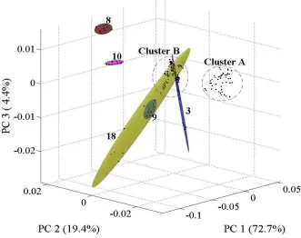
Figure 2.6 PCA scores plot of 39 brown polyester fibers with 95% elliptical

confidence regions around clustered samples removed ...65

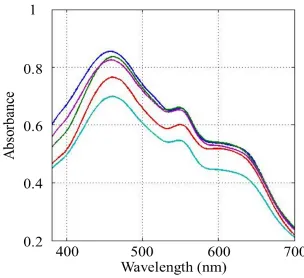
Figure 2.7 Averaged UV-Vis absorbance spectra for five brown polyester samples in Cluster B ...66

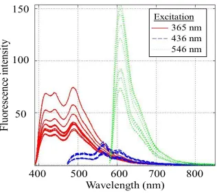
Figure 2.8 Replicate fluorescence spectra of brown polyester sample at three excitation wavelengths. Excitation at 405 nm not shown due to amount of overlap with 436 nm excitation ...67

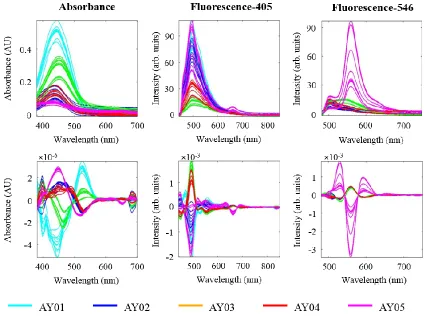
Figure 2.9 Visible absorbance and fluorescence (405 and 546 nm excitations) spectra of five yellow acrylic fibers before (top) and after (bottom) second

derivative preprocessing followed by mean centering. ...68

Figure 2.10 PCA scores plots resulting from absorbance (top left), fluorescence with 405 nm excitation (top right), fluorescence with 546 nm excitation (bottom left), and fusion of all three techniques (bottom right) for nine Purplce cotton fibers. ...69

Figure 3.1 Schematic of the methodology used for the classification of combined

laboratory datasets ...95

Figure 3.2 Microscopic images of 12 blue acrylic fibers under 40× magnification ...96

Figure 3.3 Mean absorbance spectra of 12 blue acrylic fibers collected at five

laboratories ...97

Figure 3.4 PCA scores plot of 12 blue acrylic samples (10 replicates each) collected at laboratory three ...98

Figure 3.5 Decision boundaries used to separate samples 086 and 112 generated by QDA (solid line), LDA using pooled-covariance from all 12 samples (dashed line), and LDA with sample 099 excluded from pooled-

covariance (dotted line). Class means are indicated by ‘X’ ...99

Figure 3.6 Classification error of LDA resulting from transfer of classification models to five laboratories. Each ‘o’ label involves that method of

(13)

xii

Figure 4.1 Absorbance spectra from magnetic tape samples (a) before preprocessing and (b) after preprocessing with Savitzky-Golay smoothing followed by standard normal variate transform and mean centering ...130

Figure 4.2 Partial least squares discriminant analysis scores plot for playable and

non-playable magnetic tape samples ...131

Figure 4.3 Partial least squares discriminant analysis loadings plot for the first three latent variables ...132

Figure 4.4 Average classification error of calibration and stratified 10-fold cross- validation models by number of latent variables used in partial least

squares discriminant analysis ...133

Figure 4.5 Three layer feed-forward artificial neural network ...134

Figure 4.6 Artificial neural network performance progress of training, validation, and test data. Best validation performance is indicated by intersecting

dashed lines ...135

Figure 4.7 Log posterior probabilities of magnetic tapes included in the calibration (left) and test (right) sets belonging to playable non-playable classes as determined by naïve Bayes classification. Blue and red markers indicate class determined by playability testing. Magenta markers indicate region of signficant overlap of classes ...136

Figure 4.8 Decision tree used to classify playable (P) and non-playable (NP) magnetic tapes using scores from 11 latent variables selected by partial least squares discriminant analysis ...137

Figure 5.1 MATSA program title window (left) and main user interface (right) ...159

Figure 5.2 MATSA spectral plot window showing examples of magnetic audio tape raw absorbance spectra (left) and spectra preprocessed using

interpolation, Savitzky-Golay smoothing, standard normal variate

transform, and mean centering (right) ...160

Figure 5.3 MATSA scores (left) and loadings (right) plots resulting from feature

Extraction by principal component analysis ...161

Figure 5.4 MATSA displays of validation accuracy with newly selected algorithms (left) and validation results for all algorithms based on the number of

(14)

xiii

Figure 5.5 MATSA displays showing samples to be predicted in the space of the first two latent variables with linear boundary separating playable tapes from non-playable tapes (left) and playability predictions for each sample in tabular form (right) ...163

Figure 5.6 MATSA three-dimensional plots showing decision planes resulting from linear discriminant analysis on the principal component scores with an equal cost of misclassifying tapes (left) and with a higher cost of falsely classifying non-playable tapes as playable (right) ...165

Figure 5.7 Dendrogram showing two clusters from hierarchical cluster analysis using Ward’s linkage on the average ATR FT-IR absorbance spectra from 41 tapes in an assorted collection listed by brand and model number ...166

Figure 5.8 Average spectra of two clusters resulting from hierarchical cluster

(15)

xiv

“The three great essentials to achieve anything worthwhile are, first, hard work; second, stick-to-itiveness; third, common sense.”

(16)

1

CHAPTER 1 COMPARISON OF MULTIVARIATE PREPROCESSING TECHNIQUES

FOR THE FORENSIC DISCRIMINATION OF COTTON FIBERS BY

UV-VISIBLE MICROSPECTROPHOTOMETRY

ABSTRACT

Color plays a critical role when analyzing natural fibers such as cotton in forensic

investigations. Ultraviolet-visible microspectrophotometry is a non-destructive technique

capable of providing objective color measurements on fibers in the form of absorption or

transmission spectra. Forensic fiber examinations are often hindered, however, by spectra

with little detail or points of comparison. In this work, samples of reactive, direct, and vat

dyed cotton fibers were analyzed and spectra were preprocessed using multiple methods

including baseline correction, normalization, and derivatives. Principal component

analysis followed by linear discriminant analysis was employed to discriminate the cotton

samples.

Direct dyed fibers exhibited almost featureless and low absorbing spectra

compared to those of reactive and vat dyed fibers. As a result, classification accuracies

for direct dyed fibers were lower than those calculated for reactive and vat dyed fibers.

The results of this study show that derivative spectra can significantly enhance structure

(17)

2

exhibited by direct dyed cotton fibers. No single method was best for all classes of fibers

in the study, and the shapes and intensities of the curves are important when determining

if derivative calculations are auspicious.

1. INTRODUCTION

Cotton is the most abundant fiber in the world with an estimated 25 million tons

produced annually.1 Much of that amount is used in clothing manufacturing.2 The

likelihood of recovering cotton fibers from a crime scene is the highest of any fiber type,

as population studies have shown cotton to be the most common textile fiber found on

indoor3,4 and outdoor surfaces5, as well as human head hair.6 Certain types of cotton

fibers, such as indigo dyed and colorless cotton, are found in such abundance that they

are often considered of little significance for use by forensic analysts.

Cotton fibers can be categorized based on the method in which they were dyed.

Fibers dyed using reactive dyes make up the majority of all cotton fibers, and their

dominance over direct and vat dyed fibers is expected to continue due to the excellent

wetfastness properties of reactive dyed fibers and the range of brilliant colors which can

be made using these dyes.7 Although the strength of the covalent bonding between

reactive dyes and the fiber allows for some superior properties, these forces also make

removing the dye from the fiber very challenging in cases where one wishes to use

chromatographic methods of analysis. Direct dyed fibers seemingly account for only

about 10% of all colored cotton fibers8, and vat dyed fibers share a similar percentage.

Due to the decreasing popularity of direct and vat dyes, the evidentiary value of fibers

(18)

3

Color-based techniques such as thin layer chromatography, Raman spectroscopy,

and ultraviolet-visible (UV-Vis) microspectrophotometry (MSP) are popular methods

used to analyze cotton fibers due to the lack of other defining characteristics in most

natural fibers.9-11 UV-Vis MSP provides a simple, non-destructive method for analyzing

fibers in situ. The technique is often beneficial for excluding fibers which are

indistinguishable by other approaches such as comparison light microscopy and

fluorescent light microscopy.12

The traditional method used to compare two fibers by UV-Vis MSP might have a

forensic examiner overlaying representative absorption or transmission spectra and

comparing them based on the locations and shapes of the peaks. Spectral preprocessing

techniques can be performed on UV-Vis data to potentially present the data in a more

useful way. For example, differentiation has been used for many years in analytical

chemistry for various applications described elsewhere.13,14 The use of derivatives has

only been used sparingly in forensics, however, for analyzing textile fibers15-18 and fiber

dyes.19,20

The aim of this work is to investigate the extent to which the ability to

discriminate cotton fibers is influenced by various multivariate preprocessing techniques.

Feature extraction by principal component analysis (PCA) will be used for the purpose of

reducing complex datasets down to the most significant variables which may not be

readily visible by examining the spectra. Classification accuracies will be obtained using

linear discriminant analysis (LDA), a technique which has been used in conjunction with

UV-Vis MSP in previous studies to discriminate colored textile fibers of cotton, acrylic,

(19)

4

2. EXPERIMENTAL

2.1Materials

Cotton fibers were collected from fabric obtained from a textile-related

manufacturer in the southeast United States. Dyeing of the fabric was performed at the

North Carolina State School of Textiles pilot facility (Raleigh, NC). A total of 121 cotton

fiber samples known to have been dyed using direct, reactive, or vat dyes were analyzed.

The fibers were then placed into the groups in Table 1.1 based on their observed color for

subsequent analysis by UV-Vis MSP.

Procedures from the Scientific Working Group on Materials Analysis

(SWGMAT) were followed for fiber analysis by UV-Vis MSP.23_{Single fibers were}

positioned on quartz slides (CRAIC Technologies, Altadena, CA, and Esco Products Inc.,

Oak Ridge, NJ) using micro tweezers. Each fiber was mounted using spectral grade

glycerin (Spectrum Chemical Mfg. Corp., Gardena, CA) and quartz cover slips.

2.2Instrumentation

UV-Vis spectra were obtained using a Quantum Detection Instrument (QDI) 1000

microspectrophotometer (CRAIC Technologies, San Dimas, CA). Data was processed

using GRAMS/AI version 700 software (Thermo Galactic, Salem, NH). The

microspectrophotometer was operated in transmission mode using a xenon light source.

A 15× collecting objective was used to focus the source light onto an area within the

diameter of the fiber samples, and replicate spectra were taken along the length of the

same fiber. Spectra were obtained by taking an average of 100 scans across a spectral

region of 200-850 nm with a bandwidth of 10 nm. Integration time for the charge coupled

(20)

5

2.3Data Analysis

Data was saved as comma separated variable (CSV) files and analyzed using

Fiber Spectrum Explorer, an in-house program written in MATLAB version 8.1 (The

Mathworks, Inc., Natick, MA). By convention, each dataset explored consisted of a

matrix with n (number of samples) rows and p (number of variables) columns. For

discrimination by multivariate analysis, wavelength ranges for all spectra were truncated

to a wavelength range of 380 to 700 nm. The spectra were then preprocessed using the

methods described below.

2.3.1Baseline Correction

It is common to have offsetting baselines from spectrum to spectrum in UV-Vis

measurements. Numerous methods are available for correcting offsetting baselines in

spectroscopy. Although there are more elaborate techniques for estimating the baseline of

a spectrum, the method used here involves a simple rescaling of each spectrum by

assuming the lowest non-zero intensity across a spectrum is in a region where there is

zero signal. That intensity is then subtracted from all other points in that spectrum. For

the purpose of discrimination, this method seemingly works at least as well as some

polynomial fitting algorithms.

2.3.2Normalization

Normalization to unit area is achieved by dividing each observation, X, in the ith

row and jth column, by the sum of the absolute value of all elements in that row, also

(21)

6 𝑋𝑖𝑗,𝑛𝑜𝑟𝑚=

𝑋_𝑖𝑗 ∑𝑛 |𝑋_𝑖𝑗|

𝑗=1 (1)

The result is the total area under the curve of each resulting vector being set equal to one.

Normalization to unit area is used to account for scaling differences arising from

variations in concentration, amount, and sample size as well as instrumental intensity

variations caused by changes in fiber thickness.

2.3.3Standard Normal Variate

The standard normal variate (SNV) transformation is a method of preprocessing

similar to that of the normalization technique described previously and is calculated using

Equation 2, where 𝑋_{𝑖𝑗,𝑆𝑁𝑉} is the SNV transformed point.25

𝑋_{𝑖𝑗,𝑆𝑁𝑉}= 𝑋𝑖𝑗− 𝑋𝑖

𝑠_𝑖 (2)

The sample mean spectrum, 𝑋𝑖, used in SNV calculations is not used in normalization to

unit area, however, and can instead be thought of as being set to zero. In addition,

normalization uses a scaling factor (1-norm for the calculation used in this study) in place

of the standard deviation, 𝑠_𝑖, of the sample-spectrum.

2.3.4Autoscale

Autoscaling is a method of preprocessing which involves subtracting the column

mean from each element of each column and dividing that result by the standard

deviation of the column, 𝑠_𝑗.

𝑋𝑖𝑗,𝑎𝑢𝑡𝑜 =

𝑋𝑖𝑗− 𝑋𝑗

𝑠𝑗

(22)

7

This results in the variance of all columns being equal to one. Because all values are

given equal weighting, small variations in the data are emphasized. When using data with

a low signal to noise ratio, however, noise and signal are treated equally, and this

approach becomes less useful.

2.3.5Derivatives

First derivatives (FDs) are an effective tool for correcting baseline offsets. By using a

normalization technique such as a normalization to unit area or SNV following a FD

calculation, a slope correction can also be gained. FD spectra of data recorded using

evenly spaced intervals along the x-axis can be obtained by calculating the difference

between two features, n and n + 1, where y is signal intensity and 𝜆 is wavelength.

𝜕𝑦 𝜕𝜆 =

𝑦𝑛+1− 𝑦𝑛

𝜆𝑛+1− 𝜆𝑛 (4)

The sharpest features in UV-Vis absorbance spectra are caused by noise in the measured

signal. This results in a decrease in the signal-to-noise ratio when the FD is calculated.

Noise enhancement by derivative spectroscopy is often dealt with by spectral smoothing

before differentiation. For all FD spectra in this study, a line was fitted to a 23 point

moving window using a least-squares approximation.

A second approach to dealing with the increasing noise amplification that is

associated with calculating derivatives is to use the gap-segment method. Unlike the FD

calculations collected by taking the difference of values over two adjacent points, the

second derivative (SD) calculations were made by calculating the derivative over a

number of variables (i.e., segments). The user can then define the number of variables

(23)

gap-8

segment combination is to try multiple combinations on one or more datasets, and select

the one which gives the best results. From this process, a gap size of 31 points and a

segment size of 35 points were used for all SD calculations in this study.

2.3.6Feature extraction and classification

After preprocessing, all sets of spectra were subjected to PCA. PCA is a technique

used to reduce the dimensionality of large data sets.26 In PCA, the original correlated

variables (wavelengths) are reduced to a new set of uncorrelated variables, or principal

components (PCs). PCs are linear combinations of the original variables and are arranged

in such a way that the first PC accounts for the largest variation in the data set, and the

amount of variance captured decreases with each successive PC. Selection of the number

of relevant PCs to be used in the models was chosen via scree plots which display the

percent variance captured by each PC. The greatest number of PCs before the captured

variance begins to level off was selected for use in LDA.

After the appropriate number of PCs are selected, LDA, a supervised

classification technique, was used to maximize the separation between groups in the

reduced PC space. This is carried out by projecting the data into the space of the

canonical variates. These axes differ from those in PCA in that they account for the

within-group and between-group variances after the groups are specified by the user.

Classification accuracies of each PCA-LDA model were determined internally using

leave-one-out cross-validation. In this cross-validation technique, LDA is performed on

the data set with one sample omitted thus becoming the training set. An attempt is then

made to allocate the omitted sample back into the training set. This process is repeated

(24)

9

each ‘unknown’ spectrum to the group of which the Mahalanobis distance27_{is the}

shortest.

3. RESULTS AND DISCUSSION

3.1 Comparing preprocessing methods for fiber analysis

The impact of using multiple forms of preprocessed UV-Vis spectra for fiber

discrimination with PCA-LDA was investigated. Though there is no hard-and-fast rule

for classifying cotton fibers based on the class of the dye, the classes themselves may

have characteristic changes in absorbance (∆A) across each spectrum as calculated using

Equation 5. Amax and Amin are the respective maximum and minimum absorbance values

in a spectrum as seen in Figure 1.1. For Gaussian-shaped curves, such as the ones

encountered in UV-Vis MSP, this calculation can serve as an indicator of the evenness of

the features across the spectra.

∆𝐴 = 𝐴𝑚𝑎𝑥 − 𝐴𝑚𝑖𝑛 (5)

Most direct dyed fibers in this study (80.8%) had values for ∆A between 0.005

and 0.020. The ∆A values for vat dyed fibers were mainly (85.7%) within a range of

0.020 and 0.130. Cotton fibers dyed using reactive dyes showed a broad range of ∆A

values. However, 89.2% of these fibers had a ∆A between 0.020 and 0.456. This suggests

that the majority of reactive dyed fibers show equal or greater absorption than vat dyed

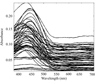
fibers. UV-Vis spectra of fibers consistent with this trend are shown in Figure 1.2.

Multivariate statistical methods were used to compare each fiber sample to other

fibers of both the same color and dye class. A group of six yellow fibers dyed using

(25)

UV-10

Vis absorbance spectra obtained for this group of fibers are shown in Figure 1.3. The

hues for these fibers were obtained using one to three dyes, the typical range for all fibers

in this study. From a visual examination of the absorbance spectra of this set of six fibers,

it was concluded that three of the fibers could easily be discriminated. As seen in Figure

1.4, the broad peaks in the averaged raw absorbance spectra of the three remaining fibers

demonstrate the challenge associated with fiber comparisons based on unprocessed

spectra. It should be noted that none of the samples in this group which appeared to have

very similar absorbance spectra shared any of the same dyes.

After all UV-Vis absorbance spectra had been preprocessed using the techniques

described in the previous section, PCA was performed to reduce the dimensionality of the

data. A requirement for LDA calculations is to have more samples than variables. If this

is not the case, inversion of the within-groups sum of squares and cross-products matrix

cannot occur. Selection of an appropriate number of PCs to include in the LDA model is

important for achieving the best separation between classes. When too many PCs are

included, the resulting classification model may generalize poorly. Overfitting is avoided

or reduced by using a Scree plot such as the one in Figure 1.5. This plot shows the

percent variance captured by each PC after performing PCA on FD spectra of the six

yellow reactive dyed fibers. Four PCs, containing 91.7% of the total variance in the data,

were chosen as the number used as input for LDA, since the variance appears to be

relatively flat for all PCs greater than four.

Table 1.2 shows the confusion matrix resulting from leave-one-out

cross-validation on the PC-LDA model of the six yellow reactive dyed fibers after FD

(26)

11

60) was obtained for the group of six yellow reactive dyed fibers after FD preprocessing.

As was already shown, samples RY03 and RY05 have very similar absorbance spectra.

The PCA scores plot in Figure 1.6 shows that even after FD preprocessing, there is still

significant overlap of the 95% confidence ellipses calculated for the two groups of fibers.

No preprocessing method used in this study allowed for complete discrimination of

samples RY03 and RY05.

The positive effect that each preprocessing method has on UV-Vis absorbance

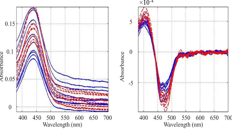
spectra is perhaps best shown using samples RY03 and RY04 (Figure 1.7). These fibers

gave very similar raw spectra, but were easily distinguishable after several types of

preprocessing. Feature by feature t-tests were used to measure the difference between the

group means at each observation point. The largest t-statistic value and the wavelength at

which it occurs are indicated following each preprocessing technique. As seen by the

t-statistic values from the raw and autoscaled spectra, autoscaling provided no

improvement in separating the two groups. In general, the changes in classification

accuracies for all groups before and after autoscaling were insignificant. Separation of the

two groups of fibers was achieved to the greatest extent by calculating SDs. This is not

surprising, as SDs correct for both baseline offsets and changes in slope. The PCA scores

plots in Figure 1.8 are consistent with the t-statistic values for each preprocessing

technique. The greatest separation between the two groups of fibers was gained using FD

(Figures 1.8g, 1.8h, and 1.8i), SD (Figure 1.8j), and SNV preprocessing techniques

(Figure 1.8d).

Classification accuracies of PCA-LDA, obtained after numerous methods of

(27)

12

Methods involving FD and SD calculations show increased classification accuracies of

direct dyed cotton fibers by as much as 11%. This gap in discrimination ability is

lessened for vat dyed fibers and is non-existent in the analysis of reactive dyed fibers.

Normalized spectra are slightly more discriminating, in the case of reactive dyed fibers,

than FD spectra. Because, in general, these fibers had larger changes in absorbance

relative to those of direct dyed fibers, this suggests there may be some cutoff value of ∆A

at which calculating derivatives provides no further benefit over using other methods of

preprocessing. The baseline correction method used in this study was found to have no

real advantage over the other preprocessing techniques used, and therefore is not

recommended. Classification accuracies for the entire dataset are shown in Table 1.4. All

FD and SD preprocessing methods used in this study, in addition to normalization, can be

considered effective methods for discriminating cotton fibers.

3.2 Fiber Spectra Comparison Tool

Using MATLAB, a Fiber Spectra Comparison Tool (FISCOTO) was developed

which would allow an examiner to view absorbance spectra of textile fibers and calculate

the previously described two sample single feature t-statistics. The design of the interface

makes the program convenient for rapidly skimming through spectra of numerous

questioned and known fibers and selecting out those fibers which require a more

thorough comparison. The user-friendly interface for the FISCOTO application is

displayed in Figure 1.9.

Spectra from multiple fibers may be loaded into FISCOTO as .CSV files.

FISCOTO uses the .CSV filenames and number of classes specified by the user to

(28)

13

Select fibers to compare list box on the left-hand side of the main user interface.

Although the user can opt to select multiple fibers to compare, a t-test for the equality of

the means is only performed when two samples are selected. The maximum t-statistic for

all features is made available for the user on the main interface. The t-statistics for all

features can be found by accessing the View t-test option located on the top right portion

of the main window.

To show an example of the single feature t-tests in FISCOTO, the same two

vat-dyed blue cotton fibers selected in Figure 1.9 will be used. After clicking the View t-test

button, the two plots in Figure 1.10 are shown. Here, the calculated t-statistics for each

feature of the raw data and data processed using Savitzky-Golay smoothing, the FD, and

standard normal variate transformation are shown in black. The horizontal green

threshold line denotes the critical value (tcrit) of Student's t at the 0.05 level of

significance, and 9 degrees of freedom (df) (due to 10 samples in each group). When the

black line is above the green line for any comparison of means at a single feature value,

the null hypothesis of equal means can be rejected at the 95% level of confidence. The

plots of calculated t-values across the feature domain also have red lines at tcalc = ~4.3,

representing a conservative choice for a threshold value. The most significant difference

between groups in the processed data is seen near 416 nm. This corresponds to the large

separation shown at that wavelength shown on the After processing panel in Figure 1.9.

In addition to hypothesis testing, this software allows users to remove undesired

features and visualize raw or processed data. FISCOTO currently makes available 12

separate methods of processing including those used in this work prior to multivariate

(29)

14

it was performed is listed in the box in the bottom right corner of the interface. This

serves as a reminder to the user as to how the data has been manipulated. The box will fill

in automatically when previously saved data is loaded back into theprogram. The Reset

option located by the Summary box undoes all performed preprocessing steps and

restores the original data.

4. CONCLUSION

Performing PCA-LDA on derivative spectra can improve discrimination of cotton

fibers over other methods of spectral preprocessing. Significant increases in

discrimination of fibers with mostly flat spectra with small changes in absorbance are

possible using derivative spectra. Direct dyed cotton fibers are one class of fibers that

would seemingly benefit significantly from utilizing derivative spectra, since these fibers

had distinctively low ∆A values. It should be noted that the effect of smoothing the

spectra using a Savitzky-Golay polynomial28 prior to calculating the FD was examined.

Although Savitzky-Golay polynomial smoothing may be advantageous for visual

examinations, increases in classification accuracies were not gained by using a

higher-order polynomial smooth rather than a linear smooth.

As was stated by Wiggins et al.19_{, there is a risk of FD spectra misclassifying}

matching fibers with large variations in absorbance. This resulted in classification

accuracies of FD spectra being slightly lower in the analysis of reactive dyed cotton

fibers when compared to the normalized spectra. Still, the high classification accuracies

(greater than 90%) achieved using all methods of preprocessing are significant due to the

difficulty of extracting these dyes for analysis by other techniques such as thin-layer

(30)

15

best for all types of spectra, a convenient software application with many preprocessing

options available, called FISCOTO, was developed for rapid comparisons of fiber

spectra. The program is freely available and can be attained by sending a request to the

author.

ACKNOWLEDGMENTS

This project was supported by Award No. 2010-DN-BX-K245 from the National

Institute of Justice, Office of Justice Programs, U.S. Department of Justice. Portions of

this work were presented at the Pittsburgh Conference on Analytical Chemistry and

Applied Spectroscopy (Pittcon) on March 6, 2014 in Chicago, IL. The co-authorship of

Jessica M. McCutcheon, John V. Goodpaster, Edward G. Bartick, and Stephen L.

Morgan is also acknowledged. The opinions, findings, and conclusions or

recommendations expressed in this presentation are those of the author(s) and do not

(31)

16 REFERENCES

1. van Dam, J. In Environmental benefits of natural fibre production and use,

Proceedings of the Symposium on Natural Fibres, Rome, Italy, 2008; pp 3-17.

2. Biermann, T.; Grieve, M. A Computerized Data Base of Mail Order Garments: a Contribution Toward Estimating the Frequency of Fibre Types Found in Clothing. Part 2: the Content of the Data Bank and its Statistical Evaluation, Forensic Sci. Int.

1996, 77, 75-71.

3. Cantrell, S.; Roux, C.; Maynard, P.; Robertson, J. A Textile Fibre Survey as an Aid to the Interpretation of Fibre Evidence in the Sydney Region, For. Sci. Int.2001, 123, 48-53.

4. Watt, R.; Roux, C.; Robertson, J. The Population of Coloured Textile Fibres in Domestic Washing Machines, Sci. Justice2005, 45, 75-83.

5. Grieve, M.; Biermann, T. The Population of Coloured Textile Fibres on Outdoor Surfaces, Sci. Justice1997, 37, 231-239.

6. Palmer, R.; Oliver, S. The Population of Coloured Fibres in Human Head Hair, Sci. Justice2004, 44, 83-88.

7. Christie, R. Colour Chemistry; Royal Society of Chemistry: Cambridge, U.K., 2001.

8. Wiggins, K. Thin Layer Chromatographic Analysis for Fibre Dyes. In Forensic Examination of Fibres, 2nd ed.; Robertson, J.; Grieve, M., Eds.; Taylor and Francis: London, U.K., 1999, pp 291-310.

9. Adolf, F.; Dunlop, J. Microspectroctrophotometry/Colour Measurement. In Forensic Examination of Fibres, 2nd ed.; Robertson, J.; Grieve, M., Eds.; Taylor and Francis: London, U.K., 1999, pp 251-289.

10.Goodpaster, J.; Liszewski, E. Forensic Analysis of Dyed Textile Fibers, Anal. Bioanal. Chem.2009, 394, 2009-2018.

11.Massonnet, G.; Buzzini, P.; Monard, F.; Jochem, G.; Fido, L.; Bell, S.; Stauber, M.; Coyle, T.; Roux, C.; Hemmings, J.; Leijenhorst, H.; Van Zanten, Z.; Wiggins, K.; Smith, C.; Chabli, S.; Sauneuf, T.; Rosengarten, A.; Meile, C.; Ketterer, S.; Blumer, A. Raman Spectroscopy and Microspectrophotometry of Reactive Dyes on Cotton Fibres: Analysis and Detection Limits, For. Sci. Int.2012, 222, 200-207.

(32)

17

13.Bosch Ojeda, C.; Sanchez Rojas, F. Recent Applications of Derivative

Ultraviolet/Visible Absorption Spectrophotometry: 2009-2011 a Review, Microchem. J.2013, 106, 1-16.

14.Karpinska, J. Derivative Spectrophotometry – Recent Applications and Directions of Developments, Talanta2004, 64, 801-822.

15.Coyle, T.; Larkin, A.; Smith, K.; Mayo, S.; Chan, A.; Hunt, N. Fibre Mapping – a Case Study, Sci. Justice2004, 44, 179-186.

16.Grieve, M.; Biermann, T.; Schaub, K. The Individuality of Fibres Used to Provide Forensic Evidence – Not all Blue Polyesters are the Same, Sci. Justice2005, 45, 13-28.

17.Grieve, M.; Biermann, T.; Schaub, K. The Use of Indigo Derivatives to Dye Denim Material, Sci. Justice2006, 46, 15-24.

18.Wiggins, K.; Palmer, R.; Hutchinson, W.; Drummond, P. An Investigation into the Use of Calculating the First Derivative of Absorbance Spectra as a Tool for Forensic Fibre Analysis, Sci. Justice2007, 47, 9-18.

19.Almeida, V.; Vargas, A.; Garcia, J.; Lenzi, E.; Oliveira, C.; Nozaki, J. Simultaneous Determination of the Textile Dyes in Industrial Effluents by the First-Order

Derivative Spectrophotometry, Anal. Sci.2009, 25, 487-492.

20.Bridge, T.; Wardman, R.; Fell, A. Novel Digital Methods for the Qualitative

Characterization of Some Acid Dyes Applied to Wool and Nylon, Analyst1985, 110, 1307-1312.

21.Morgan, S.; Niewland, A.; Mubarak, C.; Hendrix, J.; Enlow, E.; Vasser, B. In

Forensic Discrimination of Dyed Textile Fibres Using UV-VIS and Fluorescence Microspectrophotometry, Proceedings of the 12th Meeting of the European Fibres Group, Prague, Czech Republic, 2004.

22.Morgan, S.; Hall, S.; Hendrix, J.; Bartick, E. In Pattern Recognition Methods for Classification of Trace Evidence Textile Fibers from UV/Visible and Fluorescence Spectra, Proceedings of the National Institute of Justice Trace Evidence Symposium, Kansas City, Missouri, 2011.

23.SWGMAT Forensic Fiber Examination Guidelines.

http://www.swgmat.org/Forensic%20Fiber%20Examination%20Guidelines.pdf (accessed May 5, 2014).

(33)

18

25.Barnes, R.; Dhanoa, M.; Lister, S. Standard Normal Variate Transformation and De-trending of Near-Infrared Diffuse Reflectance Spectra, Appl. Spectrosc.1989, 43, 772-777.

26.Gemperline, P. Principal Component Analysis, 2nd ed.; Gemperline, P., Ed.; Taylor & Francis: Florida, 2006, pp 69-104.

27.Mahalanobis, P. On the Generalized Distance in Statistics, Proc. Nat. Instit. Sci. India

1936, 2, 49-55.

(34)

19

Table 1.1 Groups of studied fibers categorized by dye and color.

Subclass Color Spectra

examined Subclass Color

Spectra examined

Direct Blue 60 Reactive Black 80

Green 60 Blue 110

Grey 50 Brown 150

Pink 30 Green 100

White 20 Grey 20

Yellow 40 Orange 40

Vat Blue 40 Pink 20

Brown 60 Purple 80

Green 70 Red 80

Pink 20 Yellow 60

(35)

20

Table 1.2 Confusion matrix for discrimination of yellow reactive dyed fibers.

Actual

Predicted RY01 RY02 RY03 RY04 RY05 RY06

RY01 10 0 0 0 0 0

RY02 0 10 0 0 0 0

RY03 0 0 8 0 0 0

RY04 0 0 0 10 0 0

RY05 0 0 2 0 10 0

(36)

21

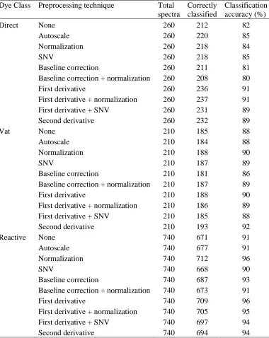
Table 1.3 Performance of PCA-LDA models following different preprocessing

techniques.

Dye Class Preprocessing technique Total

spectra

Correctly classified

Classification accuracy (%)

Direct None 260 212 82

Autoscale 260 220 85

Normalization 260 218 84

SNV 260 218 85

Baseline correction 260 211 81

Baseline correction + normalization 260 208 80

First derivative 260 236 91

First derivative + normalization 260 237 91

First derivative + SNV 260 231 89

Second derivative 260 232 89

Vat None 210 185 88

SNV 210 187 89

Second derivative 210 193 92

Reactive None 740 671 91

SNV 740 668 90

(37)

22

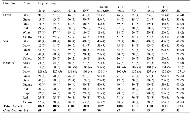
Table 1.4 Correctly classified spectra in each fiber dye class and color based category, with the number of principal components used

for each model in parentheses, following different preprocessing techniques.

Dye Class Color Preprocessing

None Autos. Norm. SNV

Baseline correction

BC +

norm. FD

FD + norm.

FD +

SNV SD

Direct Blue 50 (6) 51 (6) 46 (6) 41 (7) 51 (6) 46 (7) 55 (4) 53 (6) 51 (4) 50 (4)

Green 43 (5) 43 (5) 50 (7) 50 (7) 46 (7) 44 (7) 49 (6) 51 (7) 48 (7) 50 (8)

Grey 44 (5) 44 (5) 43 (6) 36 (7) 42 (6) 39 (8) 47 (5) 49 (4) 46 (5) 50 (8)

Pink 29 (7) 29 (7) 28 (6) 26 (6) 25 (6) 27 (6) 30 (5) 30 (5) 29 (5) 29 (5)

White 17 (4) 17 (4) 19 (6) 19 (6) 18 (4) 18 (5) 20 (5) 20 (4) 20 (5) 19 (2)

Yellow 34 (7) 34 (7) 32 (7) 32 (8) 29 (6) 34 (8) 35 (7) 37 (7) 37 (7) 34 (5)

Vat Blue 40 (4) 40 (4) 40 (4) 40 (6) 40 (4) 39 (4) 40 (5) 40 (5) 40 (5) 40 (3)

Brown 42 (5) 41 (5) 40 (5) 41 (7) 38 (5) 43 (8) 44 (8) 43 (6) 43 (8) 50 (6)

Green 63 (5) 63 (5) 69 (5) 66 (5) 63 (5) 65 (5) 63 (5) 62 (5) 62 (5) 64 (8)

Pink 20 (4) 20 (4) 19 (3) 20 (4) 20 (5) 20 (6) 20 (5) 20 (5) 19(6) 20 (2)

Yellow 20 (3) 20 (3) 20 (2) 19 (2) 19 (3) 20 (4) 20 (3) 20 (3) 20 (3) 19 (3)

Reactive Black 74 (6) 75 (5) 76 (6) 77 (7) 77 (6) 78 (5) 77 (5) 74 (5) 76 (5) 75 (5)

Blue 95 (6) 98 (5) 108 (5) 102 (4) 98 (5) 103 (4) 107 (5) 101 (5) 104 (5) 103 (5)

Brown 129 (5) 127 (5) 138 (4) 108 (4) 131 (4) 105 (5) 137 (3) 137 (4) 126 (3) 137 (6)

Green 89 (4) 90 (4) 96 (4) 91 (6) 91 (4) 94 (6) 93 (4) 97 (4) 96 (3) 92 (5)

Grey 20 (3) 20 (3) 19 (4) 19 (6) 20 (3) 19 (6) 20 (2) 20 (2) 20 (2) 20 (2)

Orange 40 (4) 40 (4) 40 (4) 40 (4) 40 (3) 40 (4) 40 (2) 40 (2) 39 (2) 40 (2)

Pink 20 (2) 20 (2) 20 (2) 20 (2) 20 (2) 20 (2) 20 (2) 20 (2) 20 (2) 20 (2)

Purple 72 (5) 74 (5) 78 (6) 79 (3) 77 (5) 78 (5) 77 (3) 78 (3) 78 (3) 77 (3)

Red 75 (5) 75 (5) 79 (5) 79 (4) 77 (4) 78 (6) 79 (5) 78 (5) 79 (5) 76 (6)

Yellow 57 (7) 58 (7) 58 (4) 53 (7) 57 (7) 58 (7) 58 (4) 58 (7) 58 (6) 58 (6)

Total Correct 1073 1079 1118 1060 1079 1068 1131 1128 1111 1123

(38)

23 0.05

0.1 0.15 0.2

A_max - A_min

400 450 500 550 600 650 700

Wavelength (nm)

Absor

ba

nc

e

(39)

24

Figure 1.2 Absorbance spectra of three cotton fibers containing A) direct blue 86 and

direct direct yellow 106, B) vat black 25, vat brown 81 and vat yellow 33, and C) reactive yellow 206.

400 450 500 550 600 650 700

0.06 0.08 0.1 0.12

Wavelength (nm)

Absor

ba

nc

e

C

B

(40)

25

Figure 1.3 Absorbance spectra of six reactive dyed yellow cotton fibers (10 replicates

each).

400 450 500 550 600 650 700

0.05 0.20

0.15

0.10

Wavelength (nm)

Absor

ba

nc

(41)

26

Figure 1.4 Averaged absorbance spectra for three of six yellow reactive dyed cotton fiber

samples.

0.16

0.12

0.05

0.04

400 450 500 550 600 650 700

Wavelength (nm)

Absor

ba

nc

e

(42)

27

Figure 1.5 Scree plot obtained following PCA on first derivative spectra of six yellow

reactive dyed cotton fibers.

2 4 6 8 10

0 5 10 15 20

Principal Component Number

V

aria

nc

e (%

(43)

28

Figure 1.6 PCA scores plot for six reactive dyed yellow cotton fibers after first derivative

preprocessing.

RY01

RY04

RY06 RY02 RY05

RY03

PC2 (13.8%)

P

C

3 (2.5

%

)

5 0

-5 -10

-4 -2 0 2 -1

(44)

29

(a) (b)

(c) (d)

(e) (f)

Figure 1.7 Absorbance spectra (10 replicates each) of samples RY03 and RY04 after a)

no preprocessing, b) autoscaling, c) normalization, d) SNV, e) baseline correction, f) baseline correction plus normalization, g) first derivative, h) first derivative plus normalization, i) first derivative plus SNV, and j) second derivative.

Wavelength (nm) A b so rb an ce

400 450 500 550 600 650 700 0.05

0.1 0.15 0.2 0.25

t-statistic = 1.4 (382 nm)

400 450 500 550 600 650 700 0.5 1 1.5 2 Wavelength (nm) A b so rb an ce

x10-3

400 450 500 550 600 650 700 0.5 1 1.5 2 A b so rb an ce Wavelength (nm) A b so rb an ce

400 450 500 550 600 650 700 -0.05

0 0.02 0.04 0.06

Wavelength (nm)

400 450 500 550 600 650 700 0

1 2 3

x10-3

Wavelength (nm) A b so rb an ce

(45)

30

(g) (h)

(i) (j)

Figure 1.7 Absorbance spectra (10 replicates each) of samples RY03 and RY04 after a)

no preprocessing, b) autoscaling, c) normalization, d) SNV, e) baseline correction, f) baseline correction plus normalization, g) first derivative, h) first derivative plus normalization, i) first derivative plus SNV, and j) second derivative.

x10-3 -4 -2 0 2 A b so rb an ce

400 450 500 550 600 700 Wavelength (nm)

650

400 450 500 550 600 650 700 -0.05 0.05 0 A b so rb an ce Wavelength (nm) t-statistic = 21.6 (504 nm)

450 500 550 600 650 x10-6 -5 0 5 A b so rb an ce Wavelength (nm) t-statistic = 25.2 (490 nm) x10-3

2

0

-2

-4

A b so rb an ce

(46)

31

(a) (b)

(c) (d)

(e) (f)

Figure 1.8 PCA scores plot resulting from absorbance spectra (10 replicates each) of

samples RY03 and RY04 after a) no preprocessing, b) autoscaling, c) normalization, d) SNV, e) baseline correction, f) baseline correction plus normalization, g) first derivative, h) first derivative plus normalization, i) first derivative plus SNV, and j) second

derivative.

PC 1 (98.2%)

-1 -0.5 0 0.5 1 1.5 -1.5 P C 2 ( 1 .6 %) -0.25 -0.2 -0.15 -0.1 -0.05 0 0.05 0.1 0.15 0.2 P C 2 ( 1 .2 %)

PC 1 (98.7%)

-10 0 10 20

-20 -3 -2 -1 0 1 2 3

PC 1 (97.6%)

PC 2 ( 1 .9 %) 0.01 0.005 0 -0.005 -0.01 -0.015 -8 -6 -4 -2 0 2 4 6 8 10 x10

-4

x10-4 -1.5 -1 -0.5 0 0.5 1 -3 -2 -1 0 1 2 3 4 P C 2 ( 3 2 .8 %)

PC 1 (52.9%)

PC 1 (90.8%)

P C 2 ( 5 .8 %) -0.06 -0.04 -0.02 0 0.02 0.04 0.06 0.08

-0.6 -0.4 -0.2 0 0.2

x10-3 x10-3 -4 -3 -2 -1 0 1 2 3 4 P C 2 ( 3 4 .2 %) PC1 (55.9%)

(47)

32

(g) (h)

(i) (j)

Figure 1.8 PCA scores plot resulting from absorbance spectra (10 replicates each) of

samples RY04 and RY05 after a) no preprocessing, b) autoscaling, c) normalization, d) SNV, e) baseline correction, f) baseline correction plus normalization, g) first derivative, h) first derivative plus normalization, i) first derivative plus SNV, and j) second

derivative.

PC 1 (44.4%)

-2 -1.5 -1 -0.5 0 0.5 1 -1 -0.5 0 0.5 1 P C 2 ( 2 9 .0 %) x10-3 x10-3

-0.01 -0.005 0 0.005 0.01 -5

-0 -5 x10

-3 P C 2 ( 1 1 .4 %)

PC 1 (56.0%)

0 0.1

0.05

-0.05

-0.1

-0.2 -0.1 0 0.1 0.2

P C 2 ( 8 .4 %)

PC 1 (56.9%) PC 1 (52.9%)

(48)

33

(49)

34

Figure 1.10 Calculated feature-by-feature t-statistics for raw (left) and processed (right)

(50)

35

CHAPTER 2 CLASSIFICATION STRATEGIES FOR FUSING UV-VISIBLE

ABSORBANCE AND FLUORESCENCE MEASUREMENTS FROM

TEXTILE FIBERS

ABSTRACT

A recent emphasis in forensic science has been placed on the development of

statistical methods for improving the interpretability of trace evidence analyses.

Determining which non-destructive analytical methods will have the highest

discrimination power for trace evidence examinations is significant to forensic

laboratories to save time and assets. Knowing which analytical techniques provide

complimentary information on the evidence is also useful for ensuring that the data

collected is utilized in the optimum manner.

This study compares the discrimination ability of ultraviolet-visible (UV-Vis)

microspectrophotometry (MSP) and microspectrofluorimetry (MSF), two common

techniques used by forensic analysts to study textile fibers. Fusion of MSP and MSF data

was also evaluated. Low-, intermediate-, and high-level data fusion strategies were

employed in discriminations of over 400 dyed textile fiber samples of cotton, acrylic,

nylon 6,6, and polyester, resulting in correct classification rates of 97.8%, 94.6%, and

93.8%, respectively. Comparatively, classification rates of 89.5%, 87.7% and 87.6%

resulted from quadratic discriminant analysis models built from isolated absorbance

(51)

36

measurements with 546 nm excitation, respectively. The results suggest that data fusion

is useful for providing additional discriminatory information on textile fibers when

compared to single technique data evaluations.

1. INTRODUCTION

Textile fibers are a frequently encountered form of class evidencein forensic

investigations of incidents involving personal contact.1,2 Cotton is the most abundant

natural source of fibers in the world3_{, and nylon, polyester, and acrylic fibers are three of}

the most common classes of synthetic fibers likely to be encountered in forensic

investigations.4 As a whole, these fibers are found as trace evidence in more than 80% of

all criminal cases pertaining to textile fibers.5

Initial fiber analysis is often carried out using forms of microscopy. Polarized

light microscopy is beneficial towards determining the polymer class (especially for

synthetic fibers), and stereomicroscopy enables an examiner to document the physical

characteristics of a fiber such as diameter, color, and luster.6,7 If the studied fibers,

however, are a metameric match, they may not be excluded as originating from the same

source. In cases such as these, further analyses can be carried out using optical

spectroscopy techniques.

Ultraviolet-visible (UV-Vis) microspectrophotometry (MSP) is a widely accepted

technique for discriminating fibers based on color.8 Color is often the most discriminating

characteristic of dyed fibers and is the only distinctive feature of many natural fibers such

as cottons due to a lack of variation in morphology.8,9 To visualize and interpret the vast

amount of data that can be collected using one or more spectroscopic techniques,

(52)

37

Data fusion is a chemometric approach which merges data from multiple sources

with the expectation that a better interpretation can be gained from the combined data in

comparison to any single sensor. Data fusion has been examined for multiple applications

in analytical chemistry and has been heavily used in the food and drink realm.10-16 A

fused data process falls into one of three categories: low-level fusion (LLF),

intermediate-level fusion (ILF), and high-level fusion (HLF). The fusion level is

determined by the stage of data processing at which fusion is carried out. LLF involves

merging the raw or preprocessed data signals of each set of input data.10,11,17 Similarly,

ILF also involves fusion at the data-level but occurs after feature selection or feature

extraction is employed.18 For this reason, ILF is also known as feature-level fusion. In

HLF, a separate model is built for each set of input data, and the responses of each model

are then “fused” together to create one final response.19

With relative ease, fusible data can be provided by modern MSP instruments

capable of collecting transmittance, absorbance, reflectance, and fluorescence

information from fibers. Though most fiber comparisons are carried out by a simple

examination of UV-Vis transmittance or absorbance spectra, microspectrofluorimetry

(MSF) is a tool often used following MSP to provide additional discriminatory

information. This is especially true in cases where the absorbance and transmittance

spectra resulting from multiple fibers appear to match. In addition to the dye components,

dye-bath additives, and the garment material may contribute to a fiber’s fluorescence

spectrum.8

This study investigates various strategies for the fusion of UV-Vis absorbance and

(53)

38

ability to discriminate these fibers was examined using multivariate classification

techniques in the form of quadratic discriminant analysis (QDA) or naïve Bayes

classification (NBC). Multivariate approaches make it possible to extract as much

information as possible from the data, and have been applied previously to color-based

discriminations of textile fibers.20,21 Lastly, the classification accuracies from fused

UV-Vis MSP and MSF data were compared to the results found using single modality.

2. EXPERIMENTAL

2.1 Materials

A total of 482 dyed textile fibers collected from various manufacturers were

examined in the study. All fibers were classified as belonging to one of four classes,

acrylic (at least 85% acrylonitrile), cotton, nylon 6,6, and polyester, based on their

polymer component. The fibers were further placed in subgroups based on perceived

color of source material to reduce the number of overall comparisons. Single fibers were

then removed from the source using razor blades and centered on quartz microscope

slides (CRAIC Technologies, Altadena, CA, and Esco Products Inc., Oak Ridge, NJ)

using micro tweezers. Spectral grade glycerin (Spectrum Chemical Mfg. Corp., Gardena,

CA) and quartz coverslips were used to mount the fibers on the slides for analysis by

MSP and MSF.

2.2 Instrumentation

UV-Vis absorbance and fluorescence spectra were acquired using a CRAIC

Technologies Quantum Detection Instrument (QDI) 1000 MSP. Data acquisition was

carried out using GRAMS/AI 7.0 (Thermo Galactic, Salem, NH). For absorbance

(54)

39

integration time for the charge coupled device (CCD) detector of ~4 ms. Fluorescence

was carried out using a mercury light source with a CCD integration time of ~200 ms.

Fluorescence spectra were acquired after 365, 405, 436, and 546 nm excitations. All

absorbance and fluorescence spectra were calculated by performing an average of 100

scans over a range of 200-850 nm with a 10 nm bandwidth.

2.3 Data Analysis

All data was analyzed using MATLAB version 8.3 (The Mathworks, Inc., Natick,

MA) and the statistics toolbox. The ‘classify’ function with discriminant types ‘quadratic’

and ‘diagquadratic’ was used to perform QDA and NBC, respectively.

2.3.1 Preprocessing

All absorbance spectra were truncated to the region of 380 to 700 nm. Truncation

of fluorescence spectra was based on the excitation cube used. The lower wavelength

cutoff was 390, 444, 470, 581 nm for 365, 405, 436, 546 nm excitation, respectively, with

an upper wavelength cutoff of 850 nm.

Further preprocessing to be performed on the datasets was dependent on whether

the preprocessed data would be analyzed individually or as part of a fused data

classification model. Preprocessing of the absorbance data to be analyzed individually

was carried out by first calculating the first derivative of each spectrum. Noise reduction

was accomplished using a Savitzky-Golay22 numerical algorithm with a second order

polynomial and nine point moving window. The first derivative is followed by a standard

normal variate transformation. Fluorescence data to be analyzed individually was

(55)

40

final preprocessing step for the individual absorbance and fluorescence datasets is mean

centering, a technique which scales each feature to a mean of zero.

Fused absorbance and fluorescence datasets were preprocessed using the second

derivative. The second derivative spectra were calculated using the gap-segment method.

In the gap-segment technique, derivatives are calculated over a number of variables (i.e.,

segments) as opposed to adjacent points. The gap, also defined by the user, is the number

of variables between the segments. Different types of spectra from multiple datasets were

examined using various gap-segment combinations. A gap size of 31 points and segment

size of 35 points were chosen as the parameters to be used based on the resulting

absorbance and fluorescence spectra which appeared to strike a balance between feature

retention and spectral smoothing. As with the single sensor data, the datasets which

would ultimately be fused are also mean centered.

2.3.2 Classification

2.3.2.1 Single Modality

Preprocessed absorbance and fluorescence spectra were subjected to principal

component analysis (PCA). Using PCA, new sets of uncorrelated variables (PCs) are

generated for each dataset.23_{The number of PCs from each set of data to be used for}

QDA was selected by plotting the variance captured by each PC (i.e., scree plots). QDA

is similar to the popularly used discriminant method, linear discriminant analysis,

developed by R. A. Fisher in 1936.24 In QDA, however, a separate variance/covariance

matrix is calculated for each group as opposed to the pooled variance/covariance matrix

used in LDA. The result of using stratified covariance matrices is a quadratic decision

(56)

41

total number of classification attempts which were performed correctly) were determined

using leave-one-out cross-validation.

2.3.2.2 Low-level Fusion

A schematic of the LLF process is shown in Figure 2.1. To avoid increased

complexity, only fluorescence measurements collected at two excitation wavelengths

(405 and 546 nm) were used in the fused data models. The original data collected

utilizing MSP and MSF was viewed as three separate n×p matrices, where n is the

number of samples and p is the number of measured wavelengths. Before fusion, p is

equal to 940, 1193, and 790 for absorbance, fluorescence-405, and fluorescence-546,

respectively. After all data has been preprocessed as described previously, the three

matrices are horizontally concatenated, generating a single matrix with n rows and 2923

(940 + 1193 + 790) columns.

In LLF, no feature extraction or selection techniques were carried out prior to

classification. Discrimination of the fiber samples in LLF was carried out utilizing the

naïve Bayes method of classification which uses probabilistic responses. The naïve Bayes

approach assumes that the features for a given class are independent (i.e., the covariance

matrices are diagonal ones). Though this assumption is generally not valid, the technique

remains a popular one due the surprisingly good results that are often obtained on

real-world datasets.25 The substantial bias generated by assuming the features of a class are

independent is usually countered by savings in variance. Classification accuracies for

fused data models were determined using 100 iterations of stratified 10-fold

Lists in a Lighthouse

Scholar Commons

Optical Spectroscopy and Chemometrics for

Discrimination of Dyed Textile Fibers and

Magnetic Audio Tapes

OPTICAL SPECTROSCOPY AND CHEMOMETRICS FOR DISCRIMINATIONS OF

DYED TEXTILE FIBERS AND MAGNETIC AUDIO TAPES

DEDICATION

ACKNOWLEDGEMENTS

ABSTRACT

M

TABLE OF CONTENTS

LIST OF TABLES

LIST OF FIGURES

CHAPTER 1

COMPARISON OF MULTIVARIATE PREPROCESSING TECHNIQUES

FOR THE FORENSIC DISCRIMINATION OF COTTON FIBERS BY

UV-VISIBLE MICROSPECTROPHOTOMETRY

CHAPTER 2

CLASSIFICATION STRATEGIES FOR FUSING UV-VISIBLE

ABSORBANCE AND FLUORESCENCE MEASUREMENTS FROM

TEXTILE FIBERS