Bayesian Detection of Expression Quantitative Trait Loci Hot Spots

(1)

INVESTIGATION

Bayesian Detection of Expression Quantitative Trait

Loci Hot Spots

Leonardo Bottolo,*,†_{Enrico Petretto,*},†_{Stefan Blankenberg,}‡_{François Cambien,}§ _{Stuart A. Cook,*},_** Laurence Tiret,§_{and Sylvia Richardson}†,††,1 *MRC Clinical Sciences Centre, Imperial College, London W12 0NN United Kingdom,†_{Department of Epidemiology and}

Biostatistics, Imperial College, London W2 1PG, United Kingdom,‡University Heart Center, D-20246 Hamburg, Germany,

§_{INSERM UMRS 937, Pierre and Marie Curie University, 75013 Paris, France, **National Heart and Lung Institute, Imperial College,}

London W2 1PG, United Kingdom, and††MRC–HPA Centre for Environment and Health, Imperial College, London-Hareﬁeld Hospital, Hareﬁeld, Middlesex UB9 6JH, United Kingdom

ABSTRACT High-throughput genomics allows genome-wide quantification of gene expression levels in tissues and cell types and, when combined with sequence variation data, permits the identification of genetic control points of expression (expression QTL or eQTL). Clusters of eQTL influenced by single genetic polymorphisms can inform on hotspots of regulation of pathways and networks, although very few hotspots have been robustly detected, replicated, or experimentally verified. Here we present a novel modeling strategy to estimate the propensity of a genetic marker to influence several expression traits at the same time, based on a hierarchical formulation of related regressions. We implement this hierarchical regression model in a Bayesian framework using a stochastic search algorithm, HESS, that efficiently probes sparse subsets of genetic markers in a high-dimensional data matrix to identify hotspots and to pinpoint the individual genetic effects (eQTL). Simulating complex regulatory scenarios, we demonstrate that our method outperforms current state-of-the-art approaches, in particular when the number of transcripts is large. We also illustrate the applicability of HESS to diverse real-case data sets, in mouse and human genetic settings, and show that it provides new insights into regulatory hotspots that were not detected by conventional methods. The results suggest that the combination of our modeling strategy and algorithmic implementation provides significant advantages for the identification of functional eQTL hotspots, revealing key regulators underlying pathways.

T

HE current focus of biological research has turned to high-throughput genomics, which encompasses large-scale data generation and a variety of integrated approaches that combine two or more -omics of data sets. An important example of integrative genomics analysis is the investigation of the genetic regulation of transcription, also called expres-sion quantitative trait locus (eQTL) or“genetical genomics” studies (Cooksonet al.2009; Majewski and Pastinen 2011). A typical eQTL analysis follows a natural structure of paral-lel regressions between the large set of q responses (i.e., expression phenotypes), and that ofpexplanatory variables

(i.e., genetic markers, often single nucleotide polymor-phism, SNPs), where p is typically much larger than the number of observationsn.

From a statistical point of view, the size and the complex multidimensional structure of eQTL data sets pose a signif-icant challenge. Not only does one wish to detect the set of important genetic control points for each response (expres-sion phenotype), includingcis- andtrans-acting control for the same transcript, but, ideally, one would wish to exploit the dependence between multiple expression phenotypes. This will facilitate the discovery of key regulatory markers, so-called hotspots (Breitlinget al.2008),i.e., genetic loci or single polymorphisms that inﬂuence a large number of tran-scripts. Identiﬁcation of hotspots can inform on network and pathways, which are likely to be controlled by major regu-lators or transcription factors (Yvert et al. 2003; Wu et al.

2008). Most importantly, there is mounting evidence that common diseases may be caused (or modulated) by changes

Manuscript received July 5, 2011; accepted for publication August 23, 2011 Supporting information is available online athttp://www.genetics.org/cgi/content/ full/genetics.111.131425/DC1.

1_{Corresponding author: Department of Epidemiology and Biostatistics, Imperial}

(2)

at a few regulatory control points of the system (i.e., hot-spots), which can cause perturbations with large phenotypic effects (Chenet al.2008; Schadt 2009).

In this article, we set out to perform hotspot and eQTL detection in an efﬁcient manner, which exploits fully the multidimensional dependencies within the genome-wide gene expression and genetic data sets. We build upon our previous work (Bottolo and Richardson 2010), where we implemented Bayesian sparse multivariate regression for continuous response to search over the possible subsets of predictors in the large 2p_{model space. For each expression}

phenotype, this corresponds to carrying out multipoint map-ping within an inference framework, Bayesian variable se-lection (BVS), where model uncertainty is fully integrated. Here, we propose a novel structure for linking parallel mul-tivariate regressions that borrows information in a hierarchi-cal manner between the phenotypes to highlight the hotspots. To be precise, we propose a new multiplicative decomposition of the joint matrix of selection probabilities

vkj that link marker j to phenotypek and demonstrate in a simulation study that this hierarchical structure and its Bayesian implementation (hierarchical evolutionary sto-chastic search or HESS algorithm) possess good character-istics in terms of sensitivity and specificity, outperforming current methods for hotspot and eQTL detection. Finally, we show the applicability of our method in two real-case eQTL studies, including animal models and human data. Our approach is broadly applicable and extendable to other high-dimensional genomic data sets and represents a first step toward a more reliable identification of functional eQTL hotspots and the underlying causal regulators.

Analysis models for eQTL data are linked to two strands of work: (i) methods for multiple mapping of QTL, where a single continuous response, referred to as a“trait,”is linked to DNA variation at multiple genetic loci by using a multivariate re-gression approach, and (ii) models that exploit the pattern of dependence between the sets of responses associated with a predictor (i.e., genetic marker). There is a vast literature on multi-mapping QTL (see the review by Yi and Shriner 2008); some of the models have been extended to the analysis of a small number of traits simultaneously (Banerjee et al.

2008; Xuet al.2008). Several styles of approaches have been adopted ranging from adaptive shrinkage (Yi and Xu 2008; Sunet al.2010) to variable selection within a composite model space framework that sets an upper bound on the number of effects (Yi et al.2007). Most of the implemented algorithms sample the regression coefficients via Gibbs sampling. How-ever, these have not been used with a substantial set of markers in the“largepsmalln”paradigm, but mostly in case of candi-date genes or in small experimental cross-animal studies. To face the challenges typical of larger eQTL studies, we have chosen to build our multi-mapping model using a recently de-veloped Bayesian sparse regression approach (Bottolo and Richardson 2010). In this approach, subset selection is imple-mented in an efficient way for vast (potentially multi-modes) model space by integrating out the regression coefficients and

by using a purposely designed MCMC variable selection algo-rithm that enhances the model search with ideas and moves inspired by evolutionary Monte Carlo algorithms.

Theﬁrst eQTL modeling approach that explicitly set out to borrow information from all the transcripts was proposed by Kendziorski et al. (2006). In the mixture over markers (MOM) method, each response (expression phenotype) yk,

1#k#q, is potentially linked to the markerjwith prob-abilitypjor not linked to any marker with probabilityp0. All

responses linked to the markerjare then assumed to follow a common distribution fj(), borrowing strength from each

other, while those of nonmapping transcripts have distribu-tion f0. Inspired by models that have been successful for ﬁnding differential expression, the marginal distribution of the data for each response yk is thus given by a mixture

model: p0f0ðykÞ þ

Pp

j¼1pjfjðykÞ. A basic assumption of the

MOM model is that a response is associated with at most one predictor. For good identifiability of the mixture, MOM requires a sufficient number of transcripts to be associated with the markers. The authors use the EM algorithm tofit the mixture model and estimate the posterior probability of mapping nowhere or to any of theplocations. By combining information across the responses, MOM is more powerful and can achieve a better control of false discovery rates (FDR) by thresholding the posterior probabilities than pure univariate differential expression methods testing each tran-script-marker pair. But as originally developed, it is not fully multivariate as it does not account for multiple effects of several markers on each expression trait.

To improve on identiﬁcation of eQTL effects, Jia and Xu (2007) formulate a unifyingq·phierarchical model in which each transcript yk, 1 # k # q, is potentially linked to the

complete set ofpmarkersXthrough a full linear model with regression coefﬁcients,bk= (bk1,...,bkj,...,bkp)T. Inspired by

Bayesian shrinkage approaches already used in conventional QTL mapping, they propose using a mixture prior on each of thebkj, also known as“spike and slab,”

b_kj

12g_kj

Nð0;dÞ þg_kjN

0;s2_j

; (1)

with a ﬁxed very smalldfor the spike and an independent prior for the variances2

j of the slab in thejth marker. They

then link theqresponses through a hierarchical model of the Bernoulli indicators gkj, establishing what we refer to as a hierarchical regression set-up. They assume that gkj

Bernoulli(vj), 1#k,#q, and givevja Dirichlet(1, 1) prior. In this model, to improve detection of transcript-marker associations, strength is borrowed across all the transcripts via the common latent probability vj. Jia and Xu (2007)

implement their hierarchical model in a fully Bayesian framework using an MCMC algorithm called BAYES, based solely on Gibbs sampling.

The high dimensionality of both gene expression and marker space has been alternatively addressed through the use of data reduction methods. In particular, Chun and Kelesx

(3)

(2009) have proposed implementing sparse partial least-squares regression (M-SPLS eQTL) on preclustered group of transcripts. M-SPLS selects markers associated with each tran-script cluster by evaluating the loadings on a set of latent components. As the dimension of each cluster is moderate, SPLS implements a multivariate formulation that takes into account the correlation between the transcripts in the same cluster. Sparsity of the latent direction vectors is achieved by imposing a combination ofL1andL2penalties, similar to the

elastic net. The tuning parameters K andh controlling the number of latent components and the convexity of the penal-ized likelihood are tuned together by cross-validation. The output of this method is the set of the regression coefﬁcients of the markers belonging to the latent vectors that are signif-icantly associated with a subset of transcripts, selected by bootstrap conﬁdence interval.

Jia and Xu’s linked regression set-up and fully Bayesian formulation is a natural starting point for eQTL detection, which shares common features with our approach. Here, we present a novel model structure and state of the art imple-mentation based upon evolutionary Monte Carlo. We report the results of a simulation study comparing our HESS method to BAYES (Jia and Xu 2007), as well as to two alternative approaches: MOM (Kendziorski et al. 2006) and M-SPLS (Chun and Kelesx 2009). Finally, we show the application of our method to two diverse genomic experi-ments in mouse and human genetic contexts.

Theory and Methods

Hierarchical related sparse regression

Let Y5fyT

k;1#k#qg then · q matrix of responses, with yk= (yk1,. . .,ykn)Tthe sequence ofnobservations of thekth

response, and letXbe then·pdesign matrix withith row

xi= (xi1,. . .,xip)T. We assume throughout thatxiis

quanti-tative. It encompasses the case of continuous biomarkers, inbred genotypes {0, 1} for recombinant inbred (RI) strains and {0, 1, 2} genotype coding for F2animal crosses or

hu-man data. A linear model for the kth response can be de-scribed by the equation

yk ¼ak1nþXbkþek;

where ais an unknown constant,1n is a column vector of

ones,bk = (bk1,. . .,bkp)T is thep ·1 vector of regression

coefﬁcients, and ek is the error term with ekNð0;s2kInÞ,

whereInis the diagonal matrix of dimensionn. BVS is

per-formed by placing a constant prior density onakand a prior on bk, which depends on a latent binary vector gk ¼

(gk1,. . .,gkj,. . .,gkp)T, wheregkj¼1 ifbkj6¼0 andgkj¼0

if bkj ¼ 0,j ¼1,. . .,p. Conditionally on the latent binary

vector, the linear model becomes

yk¼ak1nþXgkbgkþek;

where bgk is the nonzero vector of coefﬁcients extracted

frombk,Xgkis the design matrix of dimensionn·pgk, with

columns corresponding togkj= 1, andpg_k[gTk1p the

num-ber of selected covariates for the kresponse. For every re-gression k, we assume that, apart from the intercept ak,X

contains no variables that would be included in every pos-sible model and that the columns of the design matrix have all been centered in 0.

Assuming independence of the q regression equations conditionally on the selected predictors modeled in theq· p latent binary matrix G¼ fgT_k;1#k#qg, the likelihood becomes

Yq

k¼1

f_n

yk;ak1nþXgkbgk;s

2

kIn

; (2)

wherefn() is then-variate normal density function. The description of the joint likelihood as the product ofq

regression equations is similar to the one proposed by Jia and Xu (2007). However, one important difference is the assignment in (2) of a regression speciﬁc error variance

s2

k, allowing for transcript-related residual heterogeneity

and making our formulation more ﬂexible. A more general model, seemingly unrelated regressions (SUR) introduces additional dependence between the responses Y through the noiseek, modeling the correlation between the residuals

of different responses (Banerjee et al. 2008). However, it becomes computational unfeasible when the size of q is large, which is typical in eQTL experiments.

Prior set-up

For a given k, we follow the same prior set-up for the regression coefﬁcients and error variance as described in Bottolo and Richardson (2010). First, we treat the intercept

ak separately, assigning it a constant prior,p(ak)} 1. Sec-ond, conditionally ongk, we assign ag-prior structure on the

regression coefﬁcients and an inverse-gamma (Inv Ga) den-sity to the residual variance

pb_kg_k;t;s2_k¼N

0;s2_ktXT_g kXgk

₂1

(3)

ps2_k¼Inv Gaðas;bsÞ; (4) with as, bs . 0, and Eðs2_kÞ ¼bs=ðas21Þ. This conjugate prior set-up has many advantages. The most important is that, for a given k, the marginal likelihood p(ykjX, gk, t)

can be written in a closed form that is particularly simple to compute once (3) and (4) are integrated out. Further-more, it allows for more efﬁcient MCMC exploration with correlated predictors than the nonconjugate case (i.e., when the variance components2

kin (3) is different from the error

variance) and it provides more accurate identiﬁcation of the high-probability models among those visited during the MCMC (George and McCulloch 1997). Finally it leads to a simple and interpretable expression, EðbkjjY;tÞ ¼ t=ð1þtÞbOLSkj withbOLSkj the ordinary least-squares solution,

(4)

The hierarchical structure on the regression coefficients is completed by specifying a hyper-prior on the scaling coefficientt,p(t). We adopt the Zellner–Siow priors struc-ture for the regression coefficients that can be thought as a scale mixture ofg-priors and an inverse-gamma prior ont,

p(t)¼Inv Ga(1/2,n/2) with heavier tails than the normal distribution, pðbkjgk;s2kÞ5Cauchyð0;ns2kðX

T

gkXgkÞ 21_Þ

. In general it has been observed (Bottolo and Richardson 2010) that data adaptivity of the degree of shrinkage con-forms better to different variable selection scenarios than assuming standardfixed values (which can be easily imple-mented by using a point mass prior fort). Since the level of shrinkage can influence the results of the variable selection procedure, in our model we force all theqregression equa-tions to share the same common t, linking the regression equations hierarchically through the variance of their non-zero coefficients.

The prior speciﬁcation is concluded by assigning a Bernoulli prior on the latent binary value gkj, p(gkjjvkj) ¼ Bernoulli

(vkj). The prior chosen forvkj is of paramount importance in BVS since it controls the level of sparsity,i.e., the associ-ation with a parsimonious set of important predictors. For a given response this task can be accomplished by specifying a common small-selection probability for all p predictors,

vkj ¼ vk and giving p(vk) ¼ Beta(ak, bk) (Bottolo

and Richardson 2010). Inducing sparsity when all the responses are jointly considered is harder because further constraints are desirable. eQTL surveys (Cookson et al.

2009) suggest that only a fraction of expression traits are under genetic regulation and the number of their control points is usually small. This can be modeled by assigning a different probability for each marker vkj ¼ vj with an

hyper-prior on vj. This solution, ﬁrst proposed by Jia and

Xu (2007) with the conjugate prior p(vj) ¼ Dirichlet(d1j, d2j), assumes that this selection probability is the same for

all the responses. However, whatever the sensible choice of the hyperparametersd1jandd2j,d1j,d2j¼1 ord1j,d2j¼0.5,

the posterior density greatly depends on the ratio between the number of transcripts associated to the marker j,qj,and the

total number the transcripts in the eQTL experiment,q, since

E(vjjY)¼(qj+d1j)/(q+d1j+d2j), whereqj¼# {j:gkj¼1}.

In such formulation, the results are thus clearly inﬂuenced by the number of responses analyzed and sparsity of each kth regression cannot be controlled in the prior speciﬁcation adop-ted forvkjofgkj.

In this article we propose a novel way of specifying the selection probability vkj to synthetize the beneﬁts of both

approaches, Bottolo and Richardson (2010) and Jia and Xu (2007). We propose decomposing this probability into its marginal effects

vjk5vk · rj (5)

with vk andrjthe“row”and“column”effect, respectively, and 0# vk#1 andrj$0, but constrained so that 0# vjk#

1. The idea behind this decomposition is to control the level of

sparsity for each rowkthrough a suitable choice of the hyper-parametersak,bkofp(vk)¼Beta(ak,bk), while the parameter rjcaptures the“relative propensity”of predictorjto inﬂuence

several responses at the same time. Large values ofrjindicate

that predictorjhas a marked inﬂuence onvjkand thus likely to be a hotspot. The adopted multiplicative formulation has some similarity to the disease mapping paradigm where the relative risk level acts in a multiplicative fashion on an expected number of cases in a binomial or Poisson disease risk model. A gamma density on thejth latent hotspot effect,

p(rj)¼Ga(c,d), withE(rj)¼c/d, complete the hierarchical structure for the decomposition (5).

We conclude this section by describing the choice of the hyperparameters forvkandrj. Since by constructionvk?rj,

E(vjk)¼ E(vk)E(rj). If we assumec ¼ d, the hotspot pro-pensity does not change thea priorirow marginal expecta-tion, E(vjk)¼ E(vk). However, it inﬂates the a priorirow

marginal variance Var(vjk) . Var(vk), with Var(vjk) ¼

Var(vk)(1 + d21) + d21E2(vk). For the speciﬁcation of

the hyperparameters ak and bk, we use the Beta-binomial

approach illustrated in Kohn et al.(2001), after marginal-izing over the column effect in (5). The two hyperpara-meters can be worked out once E(pgk) and Var(pgk), the

expected number and the variance of the number of ge-netic control points for each response, are speciﬁed.

Posterior inference

After integrating out the intercepts, the regression coefﬁ -cients and the error variances, the joint density can be factorized as

pðY;X;G;V;tÞ5pðYjX;G;tÞpðGjVÞpðVÞpðtÞ; (6) where pðYjX;G;tÞ5Qq_k₅₁pðykjX;gk;tÞ, pðGjVÞ5

Qq k51

Qp

j51pðgkjjvkjÞ, and pðVÞ5

Qq k¼1pðvkÞ

Qp

j¼1pðrjÞ.

Pos-terior inference is carried out on the q · p latent binary matrixG= {gkj, 1#k#q, 1#j#p}, on theq·pselection probability matrixV= {vkj, 1#k#q, 1#j#p}, and on the scaling coefﬁcientt, if notﬁxed.

Sampling G is extremely challenging since complex de-pendence structures in theXcreate well-known problems of multimodality of the model space even for a single regres-sion equation. Here the computational challenge is higher since we are aiming to explore a huge model space of di-mension (2p₎q_{. For this reason vanilla MCMC (MC}3_{, Gibbs}

sampler, simple dimension changing moves) cannot guaran-tee a reliable exploration of the model space in a limited number of iterations. In this article we use a sampling scheme introduced by Bottolo and Richardson (2010), evo-lutionary stochastic search (ESS) as a building block for our new algorithm HESS. For each response, HESS relies on running multiple chains with different“temperature”in par-allel, which exchange information about the set of covari-ates that are selected in each chain. Since chains with higher temperaturesﬂatten the posterior density, global moves (be-tween chains) allow the algorithm to jump from one local

(5)

mode to another. Local moves (within chains) permit the

fine exploration of alternative models, resulting in a com-bined algorithm that ensures that the chains mix efficiently and do not become trapped in local modes. Specific modifi -cations of ESS were introduced to comply with the structure ofvkj, which are sampled with the decomposition (5) rather than integrating them out as in ESS. This requires some modifications in the local moves (details in Supporting In-formation,File S1, Section S.2.2.)

For sampling the selection probability matrix V, we implemented a Metropolis-within-Gibbs algorithm for each element of the row effect v ¼ (v1, . . ., vq)T and column

effects r¼(r1,. . .,rq)T, rejecting proposed values outside

the range [0, 1]. However, since the dimension ofvandr is very large, tuning the proposal for each element of the two vectors is prohibitive. To make HESS fully automatic, we use the adaptive MCMC scheme proposed by Roberts and Rosenthal (2009), where the variance of the proposal density is tuned during the MCMC to reach a speciﬁed acceptance rate. To satisfy the asymptotic convergence of the adaptive MCMC scheme, mild conditions are imposed (details inFile S1, Section S.2.3).

If notfixed, the scaling coefficientt, which is common for all theqregression equations and all theLchains, is sampled using a Metropolis-within-Gibbs algorithm with random walk proposal andfixed proposal variance (details inFile S1, Section S.2.4).

Finally, we describe a complete sweep of our algorithm. We assume that the design matrix is fully known. If missing values are present, these can be imputed in a preprocessing imputation step (for instance using the ﬁll.geno function from theqtlR package for genetic crosses (Broman and Sen 2009) orFastPhase(Scheet and Stephens 2006) for human data). Without loss of generality, we assume that the responses and the design matrix have both been centered. The same notation is used when tis ﬁxed or given a prior distribution. For simplicity of notation we do not index var-iables by the chain index, but we emphasize that the de-scription below applies to each chain:

• Given Vand twe updategk, according to the ESS pro-cedure, using global and local moves. During the burn-in, we sample the latent binary vectorgkfor eachkto tune the regression speciﬁc temperature ladder (details inFile S1, Section S.2.5). After the burn-in, at each sweep, we select at random without replacement a fractionfof the regressions where to updategk.

• Given Gandt, we samplevandrwith a random walk Metropolis with adaptive proposals.

• Given G and V, we sample t with a random walk Me-tropolis with aﬁxed proposal. To balance the number of updates of the latent binary valuesgkjwith those of the scaling coefﬁcient, at each sweep, the number of times we sampletis proportional toq·p·L.

The Matlab implementation of the HESS algorithm is available upon request from the authors.

Postprocessing analysis

In this section we present some of the postprocessing operations required to extract useful information from the rich output of our model. We stress that, while here for simplicity we are not using the output of the heated chains, following Gramacy et al. (2010), posterior inference could also be carried out using the information contained in all the chains.

The primary quantity of interest is the posterior pro-pensity of each predictor to be a hotspot. In the spirit of cluster detection rules in disease mapping (Richardsonet al.

2004), we use tail posterior probabilities of the propensities

rj,i.e., declare thejth predictor to be a hotspot if Pr

r_j.1Y

$t; (7)

wheretis a chosen threshold. We have found by empirical exploration and simulations that choosing a posterior threshold oft¼0.8 gives good performance across different scenarios with varying dimensions (data not shown).

The next quantity of interest is the posterior probability of inclusion for the pair (k, j). Following Petretto et al.

(2010), themarginal probability of inclusion is

pgkj51yk

5C_k21X S

s51

1_ð_gðsÞ kj¼1Þ

ðgkÞpðgðsÞk jykÞ; (8)

where gð_ksÞ¼ ðgð_ks₁Þ;. . .; gð_kjsÞ;. . . ;gð_kqsÞÞis the latent binary vec-tor sampled at iteration s,pðgð_ksÞjykÞis the model posterior

probability obtained through inexpensive numerical integra-tion in the full output (see File S1, Section S.3) and

Ck¼

PS s¼1pðg

ðsÞ

k jykÞ is the constant of normalization. The

Bayes factor (BF) for the pair (k,j) is derived from (8) as the ratio between posterior odds and prior odds

BFkj¼

pðgkj¼1jykÞ

12pðg_kj¼1ykÞÞ

= E

pgk

=

p 12 E pgk

=

p

; (9)

where E(pgk) is the a priori expected number of genetic

control points for thekth transcript.

Similarly to (8), if of interest, we can further evaluate the joint posterior probability of the set of predictors declared as hotspots as

pð \H

j¼1ðgkj¼1ÞykÞ ¼C

21

k XS

s¼1

1_\H j¼1ðgkj¼1Þ

_ð_g

kÞpðgðsÞk jykÞ

(10) with Ck _{as before and} _H _{the set of markers identi}_ﬁ_{ed as}

hotspots.

Finally, thebest model visitedis deﬁned as

gB_k ¼

n

gðsÞ_k :max

s pðg ðsÞ k jykÞ

o

(6)

Note that the conﬁguration posterior probabilityp(GjY) (see File S1, section S.3) can be used as an alternative weight in (8) and (10) or to derive the maxa posteriori (MAP) conﬁ g-uration visited

GB¼

n

GðsÞ:max

s pðG ðsÞ_j_Y_Þo_:

Results

Simulation studies

We carried out a simulation study to compare our algorithm with recently proposed multiple response models: MOM (Kendziorskiet al.2006), BAYES (Jia and Xu 2007), and M-SPLS (Chun and Kelesx2009).

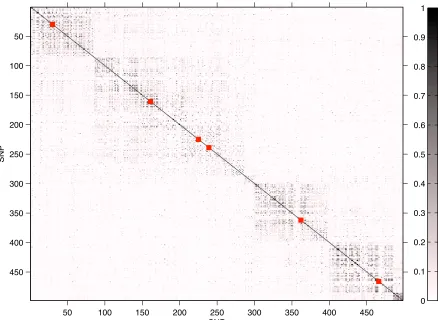
To create more realistic examples, we decided not to simulate theXmatrix, but to use real human-phased geno-type data spanning 500 kb, region ENm014 (chromosome 7: 126,368,183–126,865,324 bp), from the Yoruba population used in the HapMap project (Altshuler et al. 2005) as the design matrix. After removing redundant variables, the set of SNPs is reduced toP¼498, withn¼120, giving a 120· 498 X matrix. As noted by Chun and Kelesx (2009), high correlations between markers might affect the performance of variable selection procedures that do not explicitly con-sider such a grouping structure. The beneﬁt of using real human data are to test competing algorithms when the pat-tern of correlation,i.e., linkage disequilibrium (LD), is com-plex and blocks of LD are not artiﬁcial, but they derive naturally from genetic forces, with a slow decay of the level of correlation between SNPs (seeFigure S1).

In the simulated examples, we carefully select the SNPs that represent the hotspots (Figure S1): (i) all hotspots are inside blocks of correlated variables; (ii) theﬁrst four SNPs are weakly dependent (r2 _, _{0.1); and (iii) the remaining}

two SNPs are correlated with each other (r2 _¼ _{0.46) and}

also linked to one of the previous simulated hotspots (r2_¼

0.52 andr2_¼_{0.44, respectively), creating a potential}

mask-ing effect difﬁcult to detect. Apart from the hotspots, no other SNPs are used to simulate transcript–SNP associations. We simulated four cases:

SIM1: In this example we simulated q ¼ 100 transcripts from the selected six hotspots, with some transcripts pre-dicted by multiple correlated markers (polygenic con-trol): for instance transcripts 17–20 are regulated by three SNPs at the same time (seeFigure S2). Altogether we simulated 94 transcript–SNP associations in 50 dis-tinct transcripts. The effects were simulated from a nor-mal density with snor-maller variance than in Jia and Xu (2007), bkj N(0,0.32_)with _ek _N₍₀_{, 0.1}2_I

n) to mimic

the smaller signal-to-noise ratio expected in genetically heterogeneous human data.

SIM2: As in the previous example, we simulated 100 responses, but there are only three hotspots with the same simulated association as before, leading to 64 transcript–

SNP associations in 30 distinct transcripts. Moreover we created potential false-positive associations by simulating transcripts 81–90 and 91–100 using a linear transformation of transcript 20 with a mild negative correlation (in the interval [20.5,20.4]) and of transcript 80 with a strong positive correlation (in the interval [0.8, 0.9]), respectively. Since we create false-positive associations, the scenario will inform on how different algorithms behave when correla-tions among some transcripts are not due to SNPs. SIM3: This simulation set-up is identical to theﬁrst scenario

for theﬁrst 100 responses, but we increase the number of simulated responses toq¼1,000, simulating the further 900 transcripts from the noise.

SIM4: This is the same as the second simulated data set for the ﬁrst 100 responses, with additional 900 responses simulated from the noise, giving altogether q ¼ 1000 responses.

We discuss here the hyperparameters set-up. Sincea pri-ori, in addition to a large effect of a SNP that is located close to the transcript (cis-eQTL), we expect only a few additional control points associated with the variation of gene expres-sion (typicallytrans-eQTL); in HESS we setE(pgk)¼2 and

Var(pgk)¼ 2, meaning the prior model size for each

tran-script response is likely to range from 0 to 6 (Petrettoet al.

2010). Following Kohn et al.(2001), weﬁxed as¼10210 andbs¼1023, giving rise to a noninformative prior on the error variance. We run the HESS algorithm for 6000 sweeps with 1000 as burn-in with three chains andu¼1/4. Com-putational time is similar for the ﬁrst two simulated exam-ples, 6 hr, and 10 times greater for the last two simulated scenarios on a Intel Xeon CPU at 3.33 GHz with 24 Gb RAM. We run BAYES for 15,000 sweeps with 5000 as burn-in, recording sampled values every 5 sweeps. The variancedof the spike component 1 is set 1024, which is 100 times lower than the noise variance. Since the code available from the authors was written in SAS/IML, we recoded their Gibbs sampler in Matlab. We used the default parameters for MOM, while in M-SPLS the two tuning parameters are obtained through cross-validation selected in the interval K ¼ 1,. . ., 10 and

h ¼ 0.01, . . ., 0.99. Each simulated example was replicated 25 times and we run the four algorithms on each replicate.

Power to detect hotspots:The identiﬁcation of the hotspots is of primary interest for all the algorithms we are comparing. In HESS using the tail posterior probability Pr(rj.1jY), we

can rank the predictors according to their propensity to be a hotspot, while in BAYES the posterior mean of the common latent probabilityvj,E(vjjY) is utilized to prioritize important

markers. In MOM the strength for a predictor to be a hotspot is not directly available but, as suggested by the authors, given a marker, it can be obtained by taking a suitable quan-tile of the transcript–marker associations distribution across responses. We use their R function get.hotspots recording the average of the distribution for each predictor. M-SPLS, after cross-validation, provides a list of latent components that

(7)

predicts most of the variability ofY. While this group cannot be interpreted directly as the list of hotspots, we use it to test the existing overlap between the simulated hotspots and the latent components. Finally, differently from the analyses pre-sented in Jia and Xu (2007) and Chun and Kelesx (2009), in the HESS power calculation, we simply rank the evidence for being a hotspot provided by each algorithm across the 25 replicates. Therefore we are not using any method-speciﬁc procedure to call a hotspot, based for instance on FDR con-siderations, that could inﬂuence the comparison results.

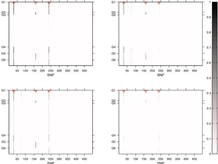
Figure 1 shows the ROC curves for the four algorithms considered. HESS (blue lines) outperforms all the other methods with sizeable power on the simulated examples. It is not signiﬁcantly affected by the dimension of the eQTL experiment (top,q¼100; bottom,q¼1000). This is some-how expected since the hotspot propensity does not depend directly on the number of transcripts analyzed (seeFile S1, section S.2.3). Spurious correlations among transcripts not due to SNPs (right) have a negligible effect on the HESS power, showing robust properties of our algorithm in detect-ing hotspots under different scenarios.

The other methods show good properties whenq¼100, but their power degrades sensibly when q¼ 1000. This is expected for BAYES (green lines) sinceE(vjjY) is affected by

q, while the performance of MOM (red lines) is more stable. MOM (red dashed lines) shows good power in the simulated examples even when the number of markers is larger than the number of traits, a situation that MOM is not designed for (top). Finally M-SPLS has greater power than BAYES, but it is outperformed by both HESS and MOM in the more sparse scenarios (bottom). Looking more closely at the list of latent vectors identiﬁed by M-SPLS (data not shown), we noted that the simulated hotspots at SNP 362 and 466 that are linked to SNP 239 were rarely selected (false negative) in both SIM1 and SIM3. On the contrary, SNP 75 is very

often included (false positive) in the list of latent vectors in all the scenarios. This might reflect the high correlation between SNP 362 and 466 with SNP 239, as well as the strong dependency between SNP 75 and 30 where we sim-ulated a hotspot. This suggests that M-SPLS has limited efficiency in the presence of complex correlation patterns in the design matrix. In Figure S3, Figure S4, Figure S5, andFigure S6, interested readers canfind the visual repre-sentation of the signals detected by each algorithm and av-eraged across the 25 replicates.

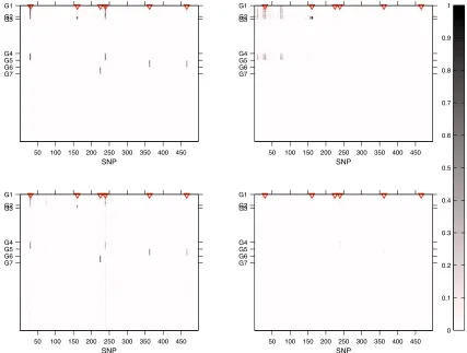
Power to detect transcript-marker associations: Figure 2 shows the ROC curves of the transcript–marker marginal associations detected by each method. Also in this case, to perform the power calculation, we are not using any method-speciﬁc way to declare a signiﬁcant association, since we sim-ply record the output from each algorithm and rank it across the 25 replicates. In particular we use the marginal probabil-ity of inclusion p(gkj = 1jyk) (8) for HESS; the posterior

frequencygkj ¼SSs¼1g

ðsÞ

kj=Sfor BAYES, whereg

ðsÞ

kj is the value

recorded at iterations; the transcript–marker association pro-vided the MOM object momObj; andﬁnally the associations selected by bootstrap conﬁdence interval at different type I error levels (a= 1024, 1023, 1022, 0.05) for M-SPLS.

For transcript–marker association detection, weﬁnd that HESS has higher power than that of the other methods in all the simulated scenarios. As expected when more responses are included, the power decreases slightly (bottom), while spurious associations due to the correlation between tran-scripts do not seem to affect the ability of HESS to distin-guish between true and false signals (right). MOM is quite stable across scenarios, but it reaches only half of the power of HESS. BAYES and M-SPLS have similar behavior and their performance degrades whenq¼1000. BAYES, in particular, has very low power since the shrinkage to the null effect,

(8)

caused by common latent probabilityvj,is particularly strong

in SIM3 and SIM4.

The different power of the methods considered can be better understood by looking atFigure S3,Figure S4,Figure S5, andFigure S6, where, for each simulated example, we averaged the evidence of transcript–marker association across replicates. HESS is able to identify the correct simu-lated pattern, with very few false positives. When false-positive associations are simulated, for instance, in SIM3 and SIM4, HESS assigns on average lower posterior probability of inclusion than for the true positive ones (Figure S4andFigure S6, top left). While MOM is able to identify the simulated hotspots, it finds it difficult to separate the true transcript– marker associations from the spurious ones (Figure S3,Figure S4,Figure S5, andFigure S6, bottom left). The main limitation of M-SPLS is the correct identification of the latent vectors when highly correlated predictors are considered (Figure S3, Figure S4,Figure S5, andFigure S6, top right). Finally BAYES is able to identify the simulated pattern whenq¼100 (Figure S3 andFigure S4, bottom right), but it seems to be too con-servative when the number of responses is large, q ¼1000 (Figure S5 and Figure S6, bottom right). The higher false-negative rate in BAYES may depend on the poor efficiency of the MCMC sampler (which is based exclusively on the Gibbs sampling that is not able to jump between distant competing models) and on the spike and slab prior that is not integrated out. The latter influences the sampling ofgkjsince the latent binary vector depends on the regression coefficients (see Figure S7for an illustration).

Real case studies

Here we present two applications of HESS to: (i) mouse gene expression data published in Lan et al.(2006) that is com-monly used as a benchmark data set for detection of eQTL (Chun and Kelesx2009) and eQTL hotspots (Kendziorskiet al.

2006; Jia and Xu 2007) and (ii) human monocytes expression

data set recently analyzed for disease susceptibility by Zeller

et al.(2010).

Mouse data set: The mouse data set has been previously described in detail (Lan et al. 2006), and it consists of 45,265 probe sets the expression of which has been mea-sured in the liver of 60 mice. Mice were collected from the F2-ob/obcross (B6 ·BTBR) and genotype data were

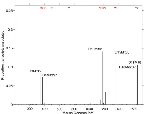
avail-able for 145 microsatellite markers from 19 autosomal chro-mosomes. To make our analysis comparable with previously reported studies (Jia and Xu 2007; Chun and Kelesx2009), we focused on 1573 probe sets showing sizeable variation in gene expression in the mouse population (sample variance .0.12). Running HESS for 12,000 sweeps with 2000 as burn-in and the same choice of the hyperparameters de-scribed in the simulation studies, among the 145 markers 16 were identified with posterior tail probability.0.8, reg-ulating a significant number of probe sets (Table S1). We report the genome location of the identified hotspots in Fig-ure 3 and show transcript–marker associations in Figure 4. Since large hotspot propensity reveals that multiple traits are controlled by the same marker, we focused on biologi-cally meaningful transcript–marker associations by using marginal probability of association .0.95 (corresponding to local FDR 5%, Ghoshet al.2006). Six markers were found to control more than 5% of all analyzed probe sets as shown in Figure 3. While marker D15Mit63 was previously detected by BAYES and M-SPLS, three other major regula-tory points were identified solely by our method: D13Mit91, D18Mit9, and D18Mit202, controlling 14.1, 10.6, and 9.7% of all analyzed probe sets, respectively (Table S2).

The regulatory hotspot at marker D13Mit91 is located within theKif13a(kinesin family member 13A) gene, which is involved in intracellular protein transport and microtu-bule motor activity via direct interaction with the AP-1 adap-tor complex (Nakagawa et al. 2000). This hotspot is

Figure 2 ROC curves for transcript–marker associations using HESS (blue line), MOM (red line), BAYES (green line), and M-SPLS (black star) in the four simulated scenarios (Figure S2). From top to bottom, left to right: SIM1,q¼ 100 and six hotspots; SIM2,q¼100 and three hotspots; SIM3,q¼1000 and six hotspots; SIM4,q¼1000 and three hotspots. For M-SPLS, power is calculated condition-ally on the list of transcript–marker associations selected by bootstrap conﬁdence interval at aﬁxed type I error (a¼

1024_{, 10}23_{, 10}22_{, 0.05). In the top, MOM is indicated by} a red dashed line to highlight that it is not designed in the cases when the number of markers is larger than the number of traits.

(9)

associated with 222 probe sets, representing 190 distinct well-annotated genes, that are enriched for speciﬁc gene ontology (GO) terms, including“protein localization”(P¼

4.2 · 1026), “protein transport” (P ¼ 5.7 · 1026), and

“establishment of protein localization” (P ¼ 6.4 · 1026). Hence, given its molecular function Kif13a is likely to be a candidate master regulator of the genes implicated with protein transport, and whose expression is associated with marker D13Mit91.

The other two newly identiﬁed markers, D18Mit9 and D18Mit202, are located on mouse chromosome 18. D18Mit9 resides within a known QTL (Hdlq30) involved in HDL cholesterol levels (Korstanje et al. 2004) whereas D18Mit202 resides within a known diabetes susceptibility/ resistance locus (Idd21, insulin-dependent diabetes suscep-tibility 21) (Hallet al.2003).

Human data set:The human data set included 648 probe sets, representing 516 unique and well-annotated genes (Ensemble GRCh37), that were found to be coexpressed in monocytes, delineating a network driven by the IRF7 tran-scription factor in 1490 individuals from the Gutenberg Heart Study (GHS) (for details on the network analysis, see Heinig et al. (2010)). This IRF7-driven inﬂammatory network (IDIN) was also reconstructed in a distinct popula-tion cohort: 758 subjects from the Cardiogenics Study show-ing signiﬁcant overlap with the network in GHS. The“core” of the network consisted of a small gene set (q ¼17), in-cludingIRF7and coregulated target genes, the expression of which was found to betrans-regulated by a locus on human chromosome 13q32 using MANOVA in Cardiogenics (Heinig

et al.2010). However, thistrans-regulation was not found in the GHS study, using similar MANOVA analysis.

Here we take a new look and use HESS to analyze the larger IDIN with 648 probe sets in the GHS population (n¼1490 individuals) and the SNP set (P¼209) spanning 1 Mb on chromosome 13q32 (data available upon request from Stefan Blankenberg under the framework of a formal-ized collaboration via a Memorandum Transfer Agreement). While MOM and BAYES fail to detect any signal at this locus, using HESS we found two SNPs, rs9557207 and rs11616269, which are detected as hotspots for the IDIN expression with tail posterior probability 0.83 and 0.91, re-spectively (Figure 5). These SNPs are located 45.3 kb (rs9557207) and 25.1 kb (rs11616269) from SNP rs9585056, which previously showed signiﬁcant trans -effect on the core gene set of the network in Cardiogenics (P¼5.0·1023). This region was also associated withEBI2

expression (P ¼ 2.2 · 1028), the candidate gene at this locus, and with type I diabetes (T1D) (P ¼ 7.0 · 10210) (Heinig et al. 2010). For the two identiﬁed hotspots, we looked in detail at each transcript–marker association and compute their BF as given in (9). We observe that 26 and 13 transcripts show clear evidence of associations (BF . 10, Kass and Raftery 2007) in the two hotspots identiﬁed (Table S3) delineating the extent of regulatory effects. To further

calibrate this evidence, we investigated BF for marker– transcript associations in a comparable simulated set-up, that of SIM3. Using the threshold BF . 10 would lead to declaring,5% false positive marker–transcript associations in the identified hotspots (data not shown). Note that most of these transcripts (80%) are found only in the network inferred in GHS and not with the Cardiogenics network, suggesting a complex pattern of regulatory effects around locus rs9585056 which is highlighted in a specific manner in each population. These population-specific regulatory effects could reflect differences in monocytes selection pro-tocols between GHS and Cardiogenics (see Heinig et al.

(2010) for details). However, the identification of hotspots at the 13q32 locus by HESS in GHS represents a significant replication of the findings previously reported, which reflects the increased power of HESS over alternative methods.

Discussion

We have presented a new hierarchical model and algorithm, HESS, for regression analysis of a large number of responses and predictors and have applied this to hotspot discovery in eQTL experiments. Simulating a variety of complex scenarios, we have demonstrated that our approach outperforms cur-rently used algorithms. In particular, HESS shows increased power to detect hotspots when a large number of transcripts are jointly analyzed. This is due to the propensity measurerj

that we use, which quantiﬁes the latent hotspot effect inde-pendently of the response dimensionality. One improvement of HESS over vanilla MCMC-based algorithms is in the search procedure that efﬁciently probes alternative models and assesses their importance, thus providing a reliable model

(10)

space exploration (Bottolo and Richardson 2010). We have also illustrated the potential of HESS to discover regulatory hotspots in two eQTL studies that encompass diverse genetic contexts (animal model and human data). In contrast to other methods, using HESS, we were able to replicate an established regulatory control of a large inﬂammatory network in humans (Heinig et al. 2010). Moreover, in the mouse data set, we identiﬁed a new candidate (Kif13a) for the regulation of a set of genes implicated in protein transport, which was not detected by other approaches.

Our model is embedded in the linear regression frame-work with additive effects. One distinct feature of our formulation is the multiplicative decomposition of the selec-tion probabilities and its hierarchical set-up, which allows other structures and/or different types of prior information to be included. For example, speciﬁc weightspkj(suitable nor-malized) could be added in (5),vjk¼vk·rj·pkj, to provide additional prior information about the regulation ofkth tran-script. This may includecis-acting genetic control or auxiliary information on regulatory effects of the jth SNP (i.e., evolu-tionary conservation, coding, noncoding, genomic location, etc.) (Leeet al.2009). Likewise, additional structure on the responses (e.g., KEGG pathways membership, predicted tar-gets of transcription factors, protein complexes, etc.) could be included using k-indexed weights, vk, to favor detection of hotspots for similar responses.

Another possible extension of our method is the inclusion of interactions in the linear model and their efﬁcient detection. Recent advances in this direction have employed either a stepwise search for interactions between prese-lected main effects (Wang et al.2011) or partition models with which to discover modules or clusters of transcript– marker responses (Zhang et al. 2010). Such approaches could be embedded in our variable selection algorithm.

The current Matlab version of HESS represents aﬁrst step toward a more efﬁcient implementation in high-level coding

languages (currently undergoing), taking advantage of the existing C++ version of ESS algorithm (Bottoloet al.2011). The approach that we propose here is ideally suited after prioritizing candidate genomic regions or gene networks, as shown in the discussed human case study. Theﬂexibility to incorporate prior biological knowledge makes our method suitable for a wide range of analyses beyond eQTL hotspots detection, including genetic regulation of miRNA targets and metabolic and epigenetic phenotypes.

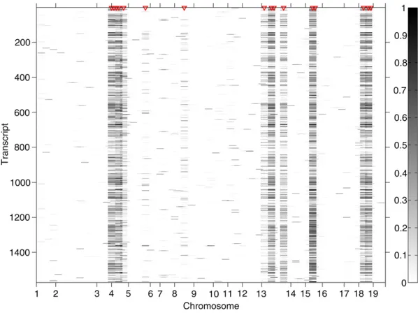
Figure 4 Heat map of the marginal probabilities of inclu-sion for each transcript–marker pair in the mouse data example (n¼60,P¼145, andq¼1573). The 16 red triangles indicate markers that have been identiﬁed as hotspots with tail posterior probability.0.8.

Figure 5 Tail posterior probability for each marker in the human data example (Gutenberg Heart Study,n¼1490,P¼209, andq¼648). Red triangles indicate markers that have been identiﬁed as hotspots with tail posterior probability.0.8. The vertical gray line highlights the physical position of annotated SNP rs9557217 and rs9585056 that were previ-ously associated with IDIN network in the Cardiogenics Study cohort and

EBI2expression (Heiniget al.2010). Thick horizontal bars on the top of theﬁgure display physical position of genes in the 1-Mb region obtained from Ensemble database.

(11)

Acknowledgments

We thank two anonymous referees and the associate editor for their comments that improved the manuscript. L.B. received funding from the Wellcome Trust Value-in-People award. S.R. gratefully acknowledges support from ESRC National Centre for Research Methods (BIAS II node, grant RES-576–25–0015). L.B. and S.R. acknowledge support from the Medical Research Council (grant G1002319). E.P. and S.A.C. acknowledge support from the Medical Research Coun-cil and the British Heart Foundation (grant FS/11/25/28740).

Literature Cited

Altshuler, D., L. D. Brooks, A. Chakravarti, F. S. Collins, M. D. Daly et al., 2005 A haplotype map of the human genome. Nature

437: 1299–1320.

Banerjee, S., B. S. Yandell, and N. Yi, 2008 Bayesian quantitative

trait loci mapping for multiple traits. Genetics 179: 2275_–2289.

Bottolo, L., and S. Richardson, 2010 Evolutionary stochastic

search for Bayesian model exploration. Bayesian Anal. 5: 583_–

618.

Bottolo, L., M. Chadeau-Hyam, D. I. Hastie, S. R. Langley, E.

Pet-rettoet al., 2011 ESS++: a C++ objected-oriented algorithm

for Bayesian stochastic search model exploration. Bioinformatics 27: 587–588.

Breitling, R., Y. Li, B. M. Tesson, J. Fu, T. Wiltshire et al.,

2008 Genetical genomics: spotlight on QTL hotspots. PLoS

Genet. 4: e1000232.

Broman, K. W., and S. Sen, 2009 A Guide to QTL Mapping with

R/qtl. Springer-Verlag, Berlin.

Chen, Y., J. Zhu, P. Y. Lum, X. Yang, S. Pinto et al.,

2008 Variations in DNA elucidate molecular networks that

cause disease. Nature 452: 429–435.

Chun, H., and S. Kelesx, 2009 Expression quantitative trait loci

mapping with multivariate sparse partial least squares regres-sion. Genetics 182: 79_–90.

Cookson, W., L. Liang, G. Abecasis, M. Moffatt, and M. Lathrop,

2009 Mapping complex disease traits with global gene

expres-sion. Nat. Rev. Genet. 10: 184_–194.

George, E. I., and R. E. McCulloch, 1997 Approaches for Bayesian

variable selection. Statist. Sinica 7: 339–373.

Ghosh, D., W. Chen, and T. Raghunathan, 2006 The false

discov-ery rate: a variable selection perspective. J. Statist. Plann.

In-ference 136: 2668–2684.

Gramacy, R. B., R. J. Samworth, and R. King, 2010 Importance

tempering. Stat. Comput. 20: 1–7.

Hall, R. J., J. E. Hollis-Moffatt, M. E. Merriman, R. A. Green, D.

Bakeret al., 2003 An autoimmune diabetes locus (Idd21) on

mouse chromosome 18. Mamm. Genome 14: 335–339.

Heinig, M., E. Petretto, C. Wallace, L. Bottolo, M. Rotival et al.,

2010 A trans-acting locus regulates an anti-viral expression

network and type 1 diabetes risk. Nature 467: 460–464.

Jia, Z., and S. Xu, 2007 Mapping quantitative trait loci for

expres-sion abundance. Genetics 176: 611_–623.

Kass, R. E., and A. E. Raftery, 2007 Bayes factor. J. Am. Stat.

Assoc. 90: 773_–795.

Kendziorski, C. M., M. Chen, M. Yuan, H. Lan, and A. D. Attie,

2006 Statistical methods for expression quantitative trait loci

(eQTL) mapping. Biometrics 62: 19–27.

Kohn, R., M. Smith, and D. Chan, 2001 Nonparametric regression

using linear combinations of basis functions. Stat. Comput. 11: 313–322.

Korstanje, R., R. Li, T. Howard, P. Kelmenson, J. Marshall et al.,

2004 Inﬂuence of sex and diet on quantitative trait loci for hdl cholesterol levels in an SM/J by NZB/BlNJ intercross popula-tion. J. Lipid Res. 45: 881–888.

Lan, H., M. Chen, J. B. Flowers, B. S. Yandell, D. S. Stapletonet al.,

2006 Combined expression trait correlations and expression

quantitative trait locus mapping. PLoS Genet. 2: e6.

Lee, S. I., A. M. Dudley, D. Drubin, P. Silver, N. J. Krogan et al.,

2009 Learning a prior on regulatory potential from eQTL data.

PLoS Genet. 5: e1000358.

Majewski, J., and T. Pastinen, 2011 The study of eQTL variations

by RNA-seq: from SNPs to phenotypes. Trends Genet. 27: 72_–

79.

Nakagawa, T., M. Setou, D. Seog, and N. Ogasawara Dohmaeet al.,

2000 A novel motor, KIF13A, transports mannose-6-phosphate

receptor to plasma membrane through direct interaction with

AP-1 complex. Cell 103: 569–581.

Petretto, E., L. Bottolo, S. R. Langley, M. Heinig, M. C. McDermott-Roeet al., 2010 New insights into the genetic control of gene expression using a Bayesian multi-tissue approach. PLOS Com-put. Biol. 6: e1000737.

Richardson, S., A. Thomson, N. Best, and P. Elliott,

2004 Interpreting posterior relative risk estimates in disease

mapping studies. Environ. Health Perspect. 112: 1016–1025.

Roberts, G. O., and J. S. Rosenthal, 2009 Examples of adaptive

MCMC. J. Comput. Graph. Statist. 9: 349–367.

Schadt, E. E., 2009 A molecular networks as sensors and drivers

of common human diseases. Nature 461: 218–223.

Scheet, P., and M. Stephens, 2006 A fast and ﬂexible statistical

model for large-scale population genotype data: applications to inferring missing genotypes and haplotypic phase. Am. J. Hum. Genet. 78: 629_–644.

Sun, W., J. G. Ibrahim, and F. Zou, 2010 Genomewide

multiple-loci mapping in experimental crosses by iterative adaptive

pe-nalized regression. Genetics 185: 349–359.

Wang, P., J. A. Dawson, M. P. Keller, B. S. Yandell, N. A. Thornberry et al., 2011 A model selection approach for expression

quan-titative trait loci (eQTL) mapping. Genetics 187: 611–621.

Wu, C., D. L. Delano, N. Mitro, S. V. Su, J. Janeset al., 2008 Gene

set enrichment in eqtl data identiﬁes novel annotations and

pathway regulators. PLoS Genet. 5: e1000070.

Xu, C., X. Wang, Z. Li, and S. Xu, 2008 Mapping QTL for multiple

traits using Bayesian statistics. Genet. Res. Camb. 91: 23–37.

Yi, N., and D. Shriner, 2008 Advances in Bayesian multiple QTL

mapping in experimental designs. Heredity 100: 240–252.

Yi, N., and S. Xu, 2008 Bayesian lasso for quantitative trait loci

mapping. Genetics 179: 1045_–1055.

Yi, N., D. Shriner, S. Banerjee, T. Mehta, D. Pompet al., 2007 An

ef_ﬁcient Bayesian model selection approach for interacting

quantitative trait loci models with many effects. Genetics 176:

1865_–1877.

Yvert, G., R. B. Brem, J. Whittle, J. M. Akey, E. Foss et al.,

2003 Trans-acting regulatory variation inSaccharomyces

cere-visiaeand the role of transcription factors. Nat. Genet. 35: 57– 64.

Zeller, T., P. Wild, S. Szymczak, M. Rotival, A. Schillert et al.,

2010 Genetics and beyond: the transcriptome of human

monocytes and disease susceptibility. PLoS ONE 5: e10693.

Zhang, W., J. Zhu, E. E. Schadt, and J. S. Liu, 2010 A Bayesian

partition method for detecting pleiotropic and epistatic eQTL modules. PLOS Comput. Biol. 6: e1000642.

(12)

GENETICS

Supporting Information

http://www.genetics.org/cgi/content/full/genetics.111.131425/DC1

Bayesian Detection of Expression Quantitative Trait

Loci Hot Spots

Leonardo Bottolo, Enrico Petretto, Stefan Blankenberg, François Cambien, Stuart A. Cook, Laurence Tiret, and Sylvia Richardson,

(13)

Bayesian Detection of eQTL Hot-spots

Supporting Information

S.1 Notation

We brieﬂy recall here the notation that was used along the paper. Moreover we introduce some

new notation to easy the the illustration of the MCMC scheme.

Let

Y

and

X

the

n

×

q

and

n

×

p

matrix of the responses and predictors, respectively. Let

Γ

=

_{

_γ

_lkj

_,

1 _≤

_l

_≤

_L,

1 _≤

_k

_≤

_q,

1 _≤

_j

_≤

_p

_}

the matrix of latent binary values, where

L

is

the number of simulated chains,

q

is the number of responses and

p

is the number of predictors

and let

Γ

k

= (

γ

1k

, . . . ,

γ

lk

, . . . ,

γ

Lk

)

T

the

L

×

p

latent binary matrix for the

k

th response in

expanded state-space, where

γ

lk

= (

γ

lk1

, . . . , γ

lkj

, . . . , γ

lkp

)

T

. Similarly let

Ω

=

{

ω

lkj

,

1 ≤

l

≤

L,

1 ≤

k

≤

q,

1 ≤

j

≤

p

}

the matrix of selection probability with

ω

lkj

=

ω

lk

×

ρ

lj

and let

Ω

k

=

(

_ω

₁_k

, . . . ,

ω

lk

, . . . ,

ω

Lk

)

T

the

L

×

p

selection matrix for the

k

th response in expanded state-space,

where

ω

lk

= (

ω

lk1

, . . . , ω

lkj

, . . . , ω

lkp

)

T

. For a given chain

l

, let

ω

l

= (

ω

l1

, . . . , ω

lk

, . . . , ω

lq

)

T

and

ρ

l

= (

ρ

l1

, . . . , ρ

lj

, . . . , ρ

lp

)

T

the ‘row’ and the ‘column’ effect, respectively. Finally the

temperature ladder for each regression equation

k

is denoted by

t

k

= (

t

1k

, . . . , t

lk

, . . . , t

Lk

)

T

with

1 =

t

1k

< t

2k

< . . . < t

Lk

.

1

(14)

S.2 Technical details of MCMC implementation

S.2.1 Full conditionals

Given (6), to sample the binary latent value

γ

lkj

, the selection probability

ω

lkj

=

ω

lk

×

ρ

lj

and

the scaling coefﬁcient

τ

, the tempered full conditionals in the expanded state-space are:

• p

(

γ

lk

| · · ·

)

∝

p

(

y

k

|

X

,

γ

lk

, τ

)

1/tlk

p_j₌₁

p

(

γ

lkj

|

ω

lkj

)

1/tlk

• p

(

ω

lk

| · · ·

)

∝

p

(

ω

lk

)

1/tlk

pj=1

p

(

γ

lkj

|

ω

lkj

)

1/tlk

• p

(

ρ

lj

| · · ·

)

∝

p

(

ρ

lj

)

q_k₌₁

p

(

γ

lkj

|

ω

lkj

)

1/tlk

• p

(

τ

| · · ·

)

∝

p

(

τ

)

L_l₌₁

q_k₌₁

p

(

y

k

|

X

,

γ

lk

, τ

)

1/tlk

Note that in the full conditional

p

(

ρ

lj

| · · ·

)

the prior density

p

(

ρ

lj

)

is not tempered and the reason

will be explained in Supporting Information S.2.3.

S.2.2 Γ

update

The update of the elements of the

q

×

p

latent binary matrix

Γ

is of paramount importance and

efﬁcient algorithms are required in order to visit the very large model space

(2

p

)

q

and to escape

from local modes. In the following we provide some technical details omitted from the main

text of the local and global moves that we found useful to implement. At each sweep of the

algorithm each/both of moves can be applied to

all

the

q

regression equations or to a random

without replacement subgroup of them (see Richardson et al. (2011) for alternative subgroup

selection with adaptive probability).

2

(15)

Local move

We ﬁrst introduce the single chain sampling scheme and then we extend the results for multiple

chains. There are many ways to update locally

γ

_k

, but we found useful to apply an extension of

Bottolo and Richardson (2010) proposal, where traditional samplers used in Bayesian variable

selection (

i.e.

MC

3

, Gibbs sampler and Reversible Jump) are replaced by a

Metropolis-within-Gibbs sampler known as Fast Scan Metropolis-Hastings (FSMH). Let

L

k(j=1)

=

p

(

y

k

|

X

,

γ

k(j=1)

, τ

)

and

L

k(j=0)

=

p

(

y

k

|

X

,

γ

k(j=0)

, τ

)

with

γ

k(j=1)

= (

γ

k1

, . . . , γ

kj

= 1

, . . . , γ

kp

)

T

and

γ

k(j=0)

=

(

_γ

_k₁

_{, . . . , γ}

_kj

= 0

_{, . . . , γ}

_kp

)

T

_{the marginal likelihood once the regression coefﬁcients}

_β

k

and

the residual error variance

σ

2k

are integrated out. Moreover let

p

(

γ

kj

= 1

|

ω

kj

) =

ω

kj

and

p

(

γ

kj

= 0

|

ω

kj

) = 1

−

ω

kj

. If a Gibbs sampler update is performed, a new value of

γ

kj

is drawn

from a Bernoulli distribution with probability

θ

kj

=

₍₁

₋

ω

kj

L

k(j=1)

ω

kj

)

L

k(j=0)

+

ω

kj

L

k(j=1)

(S.1)

if, in the previous iteration,

γ

kj

= 0

since by independence

p

(

γ

kj

= 1

|

γ

k\j

,

ω

k

) =

p

(

γ

kj

=

1 _|

_ω

_kj

)

(with an obvious modiﬁcation if

γ

kj

= 1

in the previous iteration). However in a sparse

framework, where

p

γk

p

, this probability is dominated by

ω

kj

and if

ω

kj

is small (because

for instance

ω

k

or

ρ

j

or both are small) also

θ

kj

will be small. For instance, it easy to show that

when

p

γk

p

and therefore by Kohn et al. (2001)

a

k

b

k

, the sampled value of

ω

k

is, on

average, very small

E

(

ω

k

|

y

k

) =

p

γk

+

a

k

p

+

a

k

+

b

k

.

It turns out that, if

γ

kj

= 0

, it is likely that also the new sampled value will be zero. Kohn et al.

(2001) propose to split the acceptance probability of the Metropolised version of (S.1) (to add a

3

(16)

new covariate in the regression)

1 _∧

ω

kj

L

k(j=1)

(1

₋

ω

kj

)

L

k(j=0)

Q

kj

(1

→

0)

Q

kj

(0

→

1)

,

where

Q

kj

(

· → ·

)

is the proposal density, into two parts: ﬁrstly, sampling a proposed value of

γ

kj

,

γ

kj∗

, from a Bernoulli distribution with probability

ω

kj

and then, if

γ

kj∗

=

γ

kj

, accept the new

value with probability

1 _∧

L

k(j=1)

L

k(j=0)

since

Q

kj

(0

→

1) =

ω

kj

and

Q

kj

(1

→

0) = 1

−

ω

kj

, with an obvious modiﬁcation if a deletion

is proposed. The advantage of this scheme is that the time consuming evaluation of the marginal

likelihood

L

kj

is limited to the set of variables where

γ

kj∗

=

γ

kj

.

The same sampling scheme can be extended to a parallel tempering set-up as illustrated in

Bottolo and Richardson (2010). In this case the Metropolis-within-Gibbs acceptance probability

of the

j

th predictor in the

k

th regression and the

l

th chain is

1 _∧

L

1/tlk

lk(j=1)

L

1/tlk

lk(j=0)

,

where

L

1/tlk

lk(j=1)

= [

p

(

y

k

|

X

,

γ

lk(j=1)

, τ

)]

1/tlk

and similarly for

L

1lk/t(jlk=0)

, since adding (deleting) a

covariate in the regression equation is proposed with probability

Q

lkj

(0

→

1 |

t

lk

) = ˜

ω

lkj

(

t

lk

)

(

Q

lkj

(1

→

0 |

t

lk

) = 1

−

ω

˜

lkj

(

t

lk

)

), with

˜

ω

lkj

(

t

lk

) =

ω

1/tlk

lkj

ω

1/tlk

lkj

+ (1

−

ω

lkj

)

1/tlk

the renormalised probability

[

p

(

γ

lkj

= 1

|

ω

lkj

)]

1/tlk

=

ω

1lkj/tlk

and

t

lk

the temperature attached to

the

k

th regression in the

l

th chain. Further discussion and advantages of this sampling scheme

over MC

3

, Reversible Jump and Gibbs sampler in a multiple chain set-up when the number of

4

(17)

predictors is very large with respect to the number of truly associated variables are presented in

Bottolo and Richardson (2010).

Global moves

We recall that global moves are bold moves that try to swap part or the whole state of two

ran-domly selected chains among the population of chains (Liang and Wong, 2000). In the following

we present the accepted probability of crossover operator (partial swap), exchange operator and

all-exchange operator (full swap).

Suppose that in the

k

th regression two new latent binary vectors

γ

_lk∗

and

γ

_rk∗

are generated

from two preselected chains,

l

and

r

, according to some crossover operator (Liang and Wong,

2000; Bottolo and Richardson, 2010). The proposed population of chains in the

k

th regression

Γ

∗

k

= (

γ

1k

, . . . ,

γ

lk∗

, . . . ,

γ

rk∗

. . . ,

γ

Lk

)

T

is accepted with probability

1 _∧

exp

{

f

(

γ

lk∗

|

ω

lk

, τ

)

/t

lk

+

f

(

γ

rk∗

|

ω

rk

, τ

)

/t

rk

}

exp

_{

_f

(

_γ

_lk

_|

_ω

_lk

_{, τ}

)

_/t

_lk

+

_f

(

_γ

_rk

_|

_ω

_rk

_{, τ}

)

_/t

_rk

_}

Q

k

(

Γ

∗k

,

Γ

k

|

Ω

k

, τ,

t

k

)

Q

k

(

Γ

k

,

Γ

k∗

|

Ω

k

, τ,

t

k

)

,

where

f

(

γ

lk

|

ω

lk

, τ

) = log(

p

(

y

k

|

X

,

γ

lk

, τ

))+

_j

log(

p

(

γ

lkj

|

ω

lkj

))

and

Q

k

(

Γ

k

,

·|

Ω

k

, τ,

t

k

)

is the

proposal density which is deﬁned as the product of the selection probability and the crossover

operator probability (Liang and Wong, 2000). The transition density depends on the selection

probabilities

Ω

k

in the

k

th regression, the scaling coefﬁcient

τ

and the

k

th regression

tempera-ture ladder

t

k

.

The exchange operator can be seen as special case of the crossover operator where the whole