Aalto University
School of Science
Master’s Programme in Computer, Communication and Information
Sciences
Oleksii Abramenko
Graph signal sampling via
reinforce-ment learning
Master’s Thesis
Espoo, October 20, 2018
Aalto University School of Science
Master’s Programme in Computer, Communication and Information Sciences
ABSTRACT OF MASTER’S THESIS Author: Oleksii Abramenko
Title: Graph signal sampling via reinforcement learning
Date: October 20, 2018 Pages: 59 Major: Machine Learning and Data Mining Code: SCI3044 Supervisor: Professor Alexander Jung
Graph signal sampling is one the major problems in graph signal processing and arises in a variety of practical applications, such as data compression, image denoising and social network analysis. In this thesis we formulate graph signal sampling as a reinforcement learning (RL) problem, which unleashes powerful methods developed recently within RL. Within our approach the signal sampling is carried out by an agent which crawls over the empirical graph and selects the most relevant graph nodes to sample, i.e., determines the corresponding graph signal values. Overall, the goal of the agent is to select signal samples which allow for the smallest graph signal recovery error. The behavior of the sampling agent is described using a policy which determines whether or not a particular node should be sampled. The policy is continuously adjusted which implies an inherent robustness to changes in the data structure.
We propose two RL-based sampling algorithms and evaluate their performance by means of illustrative numerical experiments. After this we conduct elaborative discussion on strengths and weaknesses of the proposed solutions and explain phenomenons observed during simulations.
Based on the simulation results, we identify some major challenges related to application of RL to graph signal sampling and propose possible solutions leading to prospects for the future work.
Keywords: machine learning, reinforcement learning, graph signal sam-pling, convex optimization, multi-armed bandit, policy gradi-ent, complex networks
Language: English
Acknowledgements
I would like to express my gratitude to Professor Alexander Jung who has enthusiastically supervised me for the last two years and not only introduced me to various machine learning methods but also greatly expanded my under-standing of this field as a whole. Membership in his research group “Machine learning for Big Data” has allowed me to obtain priceless research experience while working on relevant machine learning problems.
I am highly indebted to all professors and staff of Aalto University, who have demonstrated exceptional level of competence and maintained high academic standards ensuring that their students get access to the state-of-art knowl-edge and forefront educational services.
Finally, I would like to thank to my family and friends who have been very supportive of me all the way through my studies and provided their help when I needed it.
Espoo, Finland
October 20, 2018 Oleksii Abramenko
Abbreviations and Symbols
GSP Graph Signal Processing
SLP Sparse Label Propagation
LASSO Least Absolute Shrinkage and Selection Operator
TV Total Variation
MDP Markov Decision Processes
MAB Multi-Armed Bandit
RL Reinforcement Learning
DRL Deep Reinforcement Learning
DQN Deep Q-Network
MSE Mean Squared Error
SBM Stochastic Block Model
RWS Random Walk Sampling
URS Uniform Random Sampling
x a vector
x a scalar
X a matrix
x[i] i-th element of the vector x
∥x∥TV total variation
∥w∥1 l1 norm
|M| cardinality
x2 element-wise square of the vector x/y element-wise division of two vectors arg max
x
f(x) find suchx that maximizes f(x)
Contents
Abbreviations and Symbols 4
1 Introduction 7
2 Machine learning for graph signal processing 10
2.1 Graph signal processing fundamentals . . . 10
2.2 Sampling graph signals . . . 13
2.3 Recovering graph signals . . . 15
2.3.1 Sparse label propagation and network Lasso . . . 15
2.3.2 Overview of other recovery methods . . . 17
3 Reinforcement learning fundamentals 18 3.1 Reinforcement learning and Markov decision processes . . . . 18
3.2 Multi-armed bandits and bandit optimization . . . 20
3.2.1 ϵ-greedy exploration . . . 21
3.2.2 Upper confidence bound action selection . . . 22
3.2.3 Gradient multi-armed bandit with stochastic policy . . 23
3.3 Q-learning . . . 24
3.4 Deep Q-network . . . 25
3.5 Policy gradient . . . 28
4 Graph signal sampling as reinforcement learning problem 31 4.1 Proposed sampling algorithm based on the stochastic MAB . . 31
4.2 Sampling algorithm based on the policy gradient . . . 35
4.3 Reward choice problem . . . 36
5 Numerical experiments 40 5.1 Simulation model . . . 40
5.2 Experiments with MAB-based sampling algorithm . . . 41
5.3 Experiments with deep reinforcement learning . . . 44
5.4 Experiments with reward choice . . . 45
6 Discussion 49
6.1 Simulation results . . . 49
6.1.1 General discussion on results . . . 49
6.1.2 Note on random walk performance . . . 51
6.2 Future work . . . 52
7 Conclusions 54
Chapter 1
Introduction
Daily activities of people all across the globe generate massive amounts of data of different forms, from text messages and audio/video recordings to the specialized data produced by the industrial applications and even scientific experiments. Due to the new technologies and services, including broadband mobile networks and cloud storages, data generation rate expands exponen-tially and in unprecedented scale. A special place in this Big Data World is occupied by the structured data, or data which can be represented as a network of elements, where close or similar in some sense elements are con-nected. One striking example of the data with such an underlying structure is a social network (i.e. Facebook), where each user has a connection to sev-eral other “friend” users. Other examples of structured data may be found in bioinformatics and chemistry (networks of atoms forming molecules and net-works of molecules forming proteins), astronomy (representing the Universe as a network of planets, stars, galaxies) and many other areas.
Intrinsic network structure of numerous real-world problems allows us to analyze them using graph theory by representing network elements as nodes of a graph and connections between them as edges. Such a representation provides a set of powerful mathematical instruments which can be applied for solving relevant problems. For example, friend recommendation in social networks, such as Facebook, can be seen as a link prediction problem [30], which is a classical problem arising in the analysis of graphs. It is impor-tant to note that such a structured network data is often redundant in many ways and can be represented in a compressed or sparse way. This can be particularly useful for dealing with data compression and recovery problems, where the whole empirical graph can be recovered from relatively small num-ber of samples. In this context, first major challenge is to select the most representative samples, i.e., nodes which carry maximum information about the whole network-structured dataset. Another issue is how to recover the
CHAPTER 1. INTRODUCTION 8
required information from this relatively small number of observations. The latter problem has been extensively studied over the recent years and several convenient and efficient mathematical formulations allowing for straightfor-ward solution have been derived. Nowadays, majority of advances are mostly focusing on improving performance and scalability of the previously proposed recovery methods. On the other hand, solution to the former problem is not straightforward (details in Section 2.2) and requires new approaches.
One of these fundamentally new approaches is reinforcement learning, a machine learning paradigm which has acquired much attention and shown great success in approaching problems which have not been solved efficiently for decades. For instance, in 2010 researchers proposed Deep Q-Network (DQN) algorithm [33] for playing popular Atari games. The success of the novel RL architecture has inspired applications of RL in a variety of new fields including natural language processing [29], robotics [54], computer vision [52] and continuous control [31].
The main objective of this thesis is to interpret graph sampling as a re-inforcement learning problem. In particular, we interpret online sampling algorithm as an artificial intelligence agent which chooses the nodes to be sampled on-the-fly. The behavior of the sampling agent is represented by a policy over a discrete set of different actions which are at the disposal of the sampling agent in order to choose the next node at which the graph signal is sampled. The ultimate goal is to learn a sampling policy which deter-mines signal samples that allow for a small reconstruction error. Our goal is to study classical RL and recently proposed deep reinforcement learning (DRL) methods and investigate their applicability to the graph signal sam-pling problem. We strongly believe that usage of reinforcement learning and especially deep reinforcement learning approaches may not only bring the graph signal sampling to the qualitatively new level but can also open new horizons for the graph signal processing (GSP) in general.
Thesis contribution
This thesis models graph signal sampling as a RL problem. Based on this modelling we devise novel graph signal sampling algorithms. We discuss design of the proposed algorithms, state-action space and reward function choice, and formulate difficulties associated with usage of RL for graph signal sampling. The usefulness of the proposed sampling methods is verified by means of illustrative numerical experiments.
CHAPTER 1. INTRODUCTION 9
Structure of the Thesis
In Chapter 2 we provide a brief review of some main concepts and results within graph signal processing, with emphasis on machine learning problems. Chapter 3 studies theoretical foundations of RL and describes key algorithms which will be used in the subsequent chapters. Our main contribution is in Chapter 4 where we design two RL algorithms for graph signal sampling. In the following Chapter 5 we conduct numerical experiments, which are discussed and analyzed in Chapter 6. Chapter 7 concludes all the work done within the master’s thesis by listing key elements of the research and highlighting its relevance.
Chapter 2
Machine learning for graph
sig-nal processing
In this chapter we present fundamentals of the GSP and the role machine learning plays in recovering signals defined over graphs. We start with formu-lating general mathematical model of the GSP, including all necessary theo-retical assumptions, followed by the description of methods and approaches used to obtain sampled and recovered signals.
2.1
Graph signal processing fundamentals
We consider datasets which can be represented using an empirical graph
G = (V,E,W). The graph G is an undirected simple graph (with no self-loops or multi-edges). The nodes i ∈ V of the empirical graph correspond to the data points, whereas the edges {i, j} ∈ E connect data points which are similar. The extent of similarity between data points is quantified by the weight matrix W ∈ R|V|×|V|. We now associate each data point i ∈ V
with the feature vector fi ∈Rd and label x[i]∈R. These data labels induce
a signal x : V → R defined over graph G (see Figure 2.1). The similarity matrix W can be obtained in numerous ways, i.e., can be provided by a human expert or calculated automatically based on the distances between data points in the feature space, for example by using inverse multiquadric kernel [38]: wij = 1 √ ∥fi−fj∥2+c2 , where cis a regularization constant.
CHAPTER 2. ML FOR GRAPH SIGNAL PROCESSING 11 i (x[i],fi) j (x[j],fj) wij
Figure 2.1: Representing a dataset via an empirical graph. Notation: x[i], x[j] – graph signal values; fi, fj – node feature vectors; wij – edge weight.
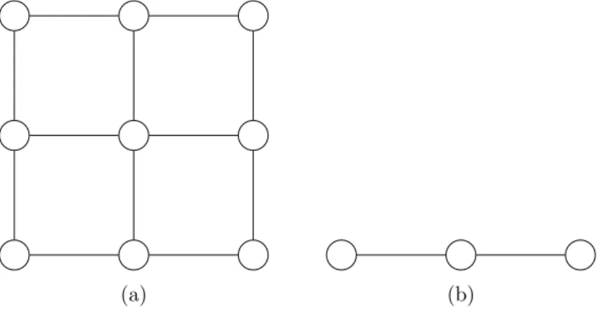
Classical examples of structured graphs are grid and chain graphs (see Figure 2.2) widely used in modern signal processing applications. For in-stance, a 2D image can be easily represented as a grid graph, with pixels being nodes and similarities between pixels being edges. The same reason-ing applies to the chain graph representation which can model time series or one-dimensional signal of any nature.
(a) (b)
Figure 2.2: Examples of network-structured datasets: (a) – grid graph rep-resenting a 2D image, (b) – chain graph reprep-resenting a time series.
In some applications the edges of the empirical graph are naturally de-fined, e.g., via friendship relations in social networks. However, sometimes it is useful to learn the network structure in a data-driven fashion. One exam-ple of such a task is a graphical model selection problem [19, 21, 36] which comes down to learning relationships between random variables in order to build conditional independence graph. Besides that, network structure learn-ing is used in many areas. For instance, Tan et. al. [42] propose data-driven network structure learning for multi-label image classification and the study [50] considers using graph learning to solve the scheduling problem.
CHAPTER 2. ML FOR GRAPH SIGNAL PROCESSING 12
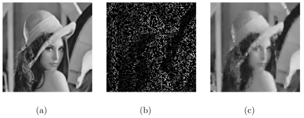
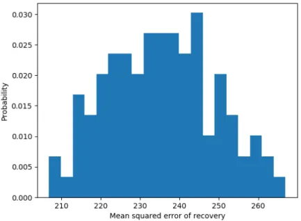
This thesis mainly revolves around graph signal sampling and recovery which are considered to be key problems in the GSP field. Extending sam-pling of time signals (e.g. audio wave signals), graph signal samsam-pling comes down to selecting a small subset of graph nodes whose signal values are rep-resentative for the entire graph signal. The dual problem to graph signal sampling is graph signal recovery. It is somewhat equivalent to the signal interpolation in the classical digital signal processing (DSP) and aims at de-termining signal values of all nodes based on signal values of nodes in the sampling set. Graph signal sampling and recovery are used together in many applications including data compression (compressing a signal using sampling and decompressing using recovery) and semi-supervised learning [2, 20]. Fig-ure 2.3 depicts example of sampling and recovering an image defined over grid graph (see Figure 2.2a). In this example we obtain sampled representa-tion by taking 25 % of all pixels uniformly at random and use it as an input to the recovery procedure described in the upcoming Section 2.3. It is worth mentioning that the recovered image does not match to the original one per-fectly and the quality of recovery powerfully depends on the sampling set choice. Furthermore, if we take 100 random sampling sets, perform recovery based on them, for each case measure mean squared error of recovery (see Section 2.2) and plot its histogram (see Figure 2.4), we can note that the difference in MSE between the best (≈ 205) and the worst (≈270) sampling sets choices amounts to approximately 30 %.
(a) (b) (c)
Figure 2.3: Example of sampling and recovering graph signal de-fined over grid graph: (a) – original graph signal, (b) – sampled graph signal, (c) – recovered graph signal. Image “Lenna” source: http://computervision.wikia.com/wiki/File:Lenna.jpg
Provided example illustrates that drawing samples to the sampling set randomly does not guarantee that the obtained sampling set will allow to reconstruct the signal with maximal quality (minimal MSE of recovery),
CHAPTER 2. ML FOR GRAPH SIGNAL PROCESSING 13
Figure 2.4: Histogram of mean squared error of graph signal recovery based on 100 random sampling sets.
therefore usage of advanced methods for finding such (sub)optimal sampling sets is necessary. In the forthcoming sections we will review existing methods for graph signal sampling and recovery and consider the most important of them in details.
2.2
Sampling graph signals
Graph signal sampling is the problem of finding a sampling setM:={i1, . . . , iM} ⊆
V of the predefined sizeM =|M|. Since acquiring signal values is often ex-pensive (requiring manual labor), the sampling set is typically much smaller than the overall dataset, i.e., M =|M| ≪N. In GSP applications we often aim at selecting such a sampling set which would lead to a minimum recon-struction error. For numeric signal values (arising in regression problems), a popular measure of the reconstruction error is the mean squared error (MSE) between recovered (conditioned on the sampling set M) ˆxM and true graph signals x: M SE:= 1 N ∑ j∈V (x[j]−xˆM[j])2
recon-CHAPTER 2. ML FOR GRAPH SIGNAL PROCESSING 14
struction method which produces ˆxM.
Graph signal sampling is related to the famous sensor selection problem [18] which considers selection of a sensor set providing the most accurate estimate of some quantity. This problem [6] as well as graph signal sampling [49] have been proven to be NP-hard, which means that in order to find optimal (in terms of minimal reconstruction error) sampling set of size M, it is required to test all (MN) combinations. Obviously that in the big data environment such an approach quickly becomes computationally intractable. Even for relatively small datasets with N = 100000 elements and M = 1000 samples, number of possible sampling set combinations reaches astronomical order of 10500. Within broad sensor selection context there is a variety of relevant methods including branch and bound search [27], convex relaxation [18], heuristic-based methods [51] and others. It should be mentioned that all these methods are either approximate or unable to deliver optimal solution in polynomial time.
Within the graph signal processing framework there is a massive amount of research which tries to address graph signal sampling problem from differ-ent perspectives. For instance, the study [9] dives deep into fundamdiffer-entals of sampling theory of the bandlimited graph signals where authors investigate performance of several graph sampling algorithms, such as uniform random sampling (URS), experimentally designed sampling and active sampling, and establish error bounds for them. Another study [43] proposes completely dif-ferent approach by handling sampling in the frequency domain and manipu-lating with Discrete Fourier Transform (DFT) of the graph. Greedy sampling selection algorithm [8] tries to find near-optimal global solution by following the sequence of locally optimal decisions.
The major drawback of almost all mentioned above graph signal sampling methods is practical impossibility to operate in the big data settings due to their overly extensive computational complexity relying on matrix decom-positions, multiplications and other computationally expensive operations. An attempt to address these scalability issues has been made in the paper [3] proposing simple and efficient algorithm based on random walk over the graph. The main idea of the algorithm is to launch random walks starting from arbitrary nodes and terminate them after sufficient number of transi-tions. The endpoints of these random walks correspond to the nodes which should be added to the sampling set. It is worth mentioning that the algo-rithm relies only on local graph information, i.e., information about neighbor-ing nodes, and does not use any computationally expensive graph representa-tions and/or mathematical operarepresenta-tions. Although the algorithm demonstrates comparable and often better performance than much more complex methods [3, Section IV], in some environments it has been found to oversample large
CHAPTER 2. ML FOR GRAPH SIGNAL PROCESSING 15
clusters and undersample small ones [1], which may sometimes lead to the performance degradation. This phenomenon will be discussed in details in the Section 6.1.2.
2.3
Recovering graph signals
In this section we consider how to recover the signal x based on observing only its samples{x[i]}i∈M. In the subsection 2.3.1 we formulate the recovery
problem as a convex optimization problem and present two popular methods to solve it, i.e., sparse label propagation (SLP) and network Lasso. In the subsection 2.3.2 we discuss other approaches used for graph signal recovery.
2.3.1
Sparse label propagation and network Lasso
The recovery of the entire graph signalxfrom (few) signal samples{x[i]}i∈M
is possible for clustered graph signals which do not vary too much over well-connected subsets of nodes (clusters) (cf. [24]). We will quantify how well a graph signal is aligned to the cluster structure using the total variation (TV)
∥x∥TV :=
∑
{i,j}∈E
Wij|x[j]−x[i]|. (2.1)
We learn the graph signal by minimizing the aforementioned total varia-tion (2.1) measure condivaria-tioning on known sampling set M:
ˆ
xM∈arg min ˜ x
∥˜x∥TV
s.t. x[i] =x[i] for all˜ i∈ M.
(2.2) The problem of the form (2.2) is known as a sparse label propagation and has been extensively studied in [24]. This is a convex optimization problem with non-differentiable objective and therefore precludes using traditional gradient-based algorithms which highly rely on derivatives. However, effi-cient method for solving (2.2) based on the primal-dual method of Cham-bolle and Pock [7] has been proposed by Jung et. al. [22]. Moreover, the study has formulated recovery procedure as a message passing, allowing for the distributed implementation which can be especially useful in the big data settings. Sometimes it can be convenient to represent total variation in the form of matrix multiplication rather than the cumulative summation (2.1). In order to do this, we convert our initial undirected graph G into its di-rected version−→G by setting orientations of edges arbitrarily. Next, we define
CHAPTER 2. ML FOR GRAPH SIGNAL PROCESSING 16
incidence matrix D ∈R|E|×|V| of the following form:
Dev := ⎧ ⎪ ⎨ ⎪ ⎩ We, v =e+ −We, v =e− 0, otherwise (2.3)
It is easy to verify that the total variation of the form (2.1) can be rede-fined using incidence matrix D in the following way:
∥x∥TV :=∥Dx∥1 (2.4)
Consequently, convex optimization problem (2.2) becomes ˆ
xM∈arg min ˜ x
∥Dx∥1
s.t. x[i] =x[i] for all˜ i∈ M.
(2.5) Presented equivalent optimization problem (2.5) can be found particularly useful when is used as an input to disciplined convex optimization solvers, such as CVX [12], which allow using only a limited number of algebraic primitives extensively optimized in terms of performance.
It should be noted that both formulations either (2.2) or (2.5) constitute constrained optimization problems. However, the unconstrained version for solving graph signal recovery can be provided as well in the form of the recently proposed network Lasso method [14, 25] which can be defined by the following convex optimization problem:
ˆ x∈arg min ˜ x λ∥x˜∥TV+ ∑ i∈M (˜x[i]−x[i])2 (2.6)
The network Lasso (2.6) conveniently separates convex optimization ob-jective into total variation and empirical error parts. The former is immedi-ately responsible for graph signal recovery itself and is identical to one in the SLP (2.2). The latter term represents an empirical error over the sampling set and penalizes deviations of the signal values being optimized from their true values. Regularization coefficient λ is an essential part of the problem and controls relative preference and impact of the terms on the optimiza-tion objective. It also helps to understand the connecoptimiza-tion between SLP and network Lasso. In particular, when λ → 0, the solution of network Lasso is drawn towards the solution of SLP. This happens because the empirical error term gets much higher preference and in order to minimize it optimization variables are forced to the same values as true labels. However, it is impor-tant to note that λ must never be 0, because in this case TV term will not
CHAPTER 2. ML FOR GRAPH SIGNAL PROCESSING 17
be able to enforce graph signal recovery on the nodes not belonging to the sampling set and graph signal at these nodes may take arbitrary values.
2.3.2
Overview of other recovery methods
Although the SLP and network Lasso described in the previous subsection are quite popular in the GSP world, here we briefly list other methods which can be used for graph signal recovery.
We start with discussing label propagation (LP) [53] which is somewhat similar to SLP presented earlier in this chapter. The key idea of the algorithm is that each node is associated with a soft label represented as a probability distribution. These labels propagate to the neighboring nodes with some probability which is proportional to the edge weights. The effect of such an operation in practice is that the label distributions of the nodes are calculated as weighted averages of the distributions of their neighbors. A fundamentally different approach is described by Romero et. al. [37] and views procedure of learning the labels from the perspective of kernel methods. The idea of this approach reduces to obtaining kernel matrix K ∈ R|V|×|V| for the
graph and then applying conventional kernel algorithms, such as kernel Ridge regression or kernel support vector machines. In their paper authors also describe several ways of obtaining kernel matrix and derive efficient numerical algorithm for solving kernel regression. This kernel-based approach has been recently extended to the Gaussian processes (GP) over graphs presented by Venkitaraman et. al. [46].
Additionally, there is a set of relatively simple and straightforward meth-ods known as average consensus and community-based labelling [32, Chapter 3]. The former method simply assigns to all the nodes such a constant which minimizes least squares error with respect to the signal values in the sampling set. This method does not take into account graph topology or any structural information and, therefore, in many cases demonstrates poor performance, but often can still be used as a baseline. The latter group of methods relies on the prior clustering by applying graph clustering or any other commu-nity detection algorithms. Then, all unlabelled nodes in each commucommu-nity are assigned signal values based on the labels of their labelled counterparts.
Chapter 3
Reinforcement learning
fundamen-tals
In this chapter we describe the main concepts and methods for solving RL problems. First, we give definition of the RL, provide a theoretical overview and compare it to the existing machine learning methods. We then briefly introduce Markov decision processes (MDP), the most fundamental reinforce-ment learning model. Second, we provide the detailed description of a simple but efficient multi-armed bandit (MAB) algorithm which will be further ref-erenced in the subsequent chapters. In Section 3.3 we describe Q-learning which is currently one of the most popular model-free RL method. Finally, the last two sections 3.4 and 3.5 focus on popular deep RL algorithms which apply deep neural networks to solve RL problems.
3.1
Reinforcement learning and Markov
de-cision processes
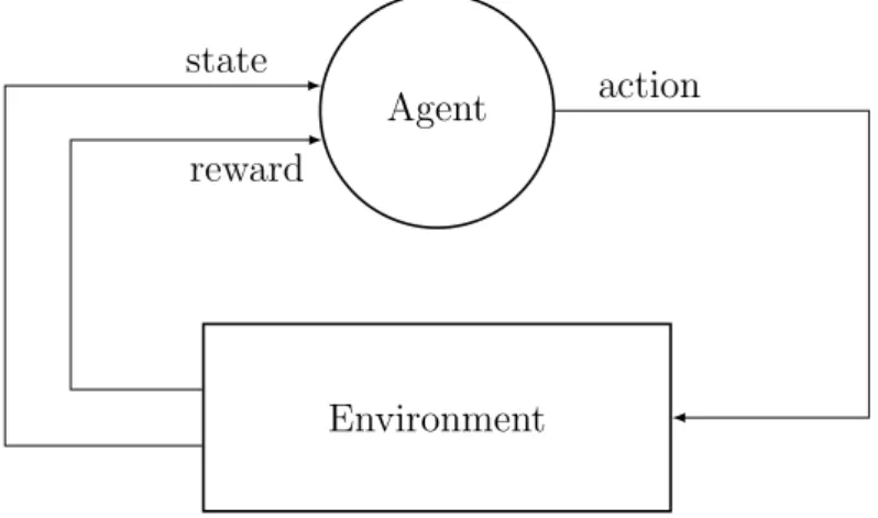
RL is a subfield of machine learning and artificial intelligence which models the process of learning through the mechanism of benefits (rewards) and punishments. RL specifies behavior of an agent in the environment, and adjusts its actions to maximize the reward. The agent interacts with the environment (see Figure 3.1) by executing actions from a predefined set and observing the response of the environment. At the following stage, the agent is more likely to choose actions which, according to its definition, have been the most successful, i.e., have resulted in the largest reward.
The action-observation procedure repeats for a sufficient number of iter-ations until the agent learns the policy – set of rules determining what to do in every possible situation.
CHAPTER 3. REINFORCEMENT LEARNING FUNDAMENTALS 19 Agent Environment reward state action
Figure 3.1: Interaction between agent and environment in reinforcement learning.
RL in general can be seen as a larger framework which incorporates dif-ferent shades of supervised and unsupervised machine learning methods. On one hand, the definition of state/action spaces and reward should be, as a rule, provided by an external supervisor. On the other hand, once these essences are known, the learning agent starts operating fully autonomously and in the unsupervised manner. In addition to this, in many applications individual supervised and unsupervised learning algorithms can be used as building blocks of a larger RL system. For instance, a robot-cleaner can use fully supervised computer vision algorithm for obstacle detection and/or recognition and then use this information as an input of the high level RL system which controls movements of the robot.
Currently, there are two major classes of RL algorithms: model-based and model-free methods. The former can be used when the environment is known, meaning that for each action taken by the agent the probability of being in a certain state is known. The latter do not assume any prior knowledge about the environment and enable learning with trial-and-error from the experience. While model-based methods are usually used in some specific applications with less demands for generalization, model-free ones often attract more attention due to their practicality and applicability to a wider range of real-world problems.
RL algorithms operate in an environment which can be described by the state space S = {si|i = 1..N} with N states and action space A =
{ai|i = 1..M} with M actions. The environment also specifies transition
CHAPTER 3. REINFORCEMENT LEARNING FUNDAMENTALS 20
when executing an action a. There is also a discount factor γ ∈ {0..1}
involved, responsible for diminishing values of rewards obtained in the far future. Based on the notation above, we introduce the simplest model-based RL approach – Markov decision process (MDP). MDP relies on the Bellman equation, estimating a quality function Q of each state-action pair:
Q(s, a) =∑
s′∈S
P(s, a, s′)(R(s, a, s′) +γQ(s′)) (3.1) The most popular algorithms for solving MDP and finding optimal policy are value iteration [4] and policy iteration methods [17]. In this thesis we do not stress much attention on them, instead we focus on more relevant to our research model-free methods described in the following sections.
3.2
Multi-armed bandits and bandit
optimiza-tion
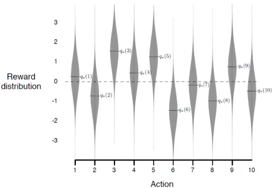
MAB is a problem of selecting the best (in the sense of maximizing reward) alternative among all available ones. The term itself originates from the notion of one-armed bandit which is an informal name of the gambling slot machine with a single lever placed on the side. In one-armed bandit settings a gambler pulls the arm and observes the reward. The reward of a particular bandit slot machine is a random variable with unknown reward distribution. In contrast to one-armed bandit case, MAB problem is defined over the environment withkone-armed bandits having their own reward distributions (see Figure 3.2). At each time step a gambler faces the decision concerning which arm to pull. The ultimate goal is to maximize the obtained reward after n consecutive arm pulls, but the major problem is that the underlying reward distributions of individual arms are unknown. Despite the fact that the exact reward distribution of i-th arm is unknown, its estimate Qi can
be obtained empirically and the best arm a can be eventually selected by maximizing estimates over arms:
Q(it)= t−1 ∑ j=1 R(j)(i) N(i) (3.2) a(t)= arg max i Q(it), (3.3)
where N(i) denotes number of times i-th arm has been pulled after total (t−1) arm pulls and R(j)(i) denotes the reward obtained on j-th time step
CHAPTER 3. REINFORCEMENT LEARNING FUNDAMENTALS 21
Figure 3.2: Example of the reward distributions of the MAB with 10 arms. q∗(1-10) denote means of the distributions. Image source: [40, Chapter 2,
Figure 2.1]
.
for the arm i. If the armi was not pulled on a certain time step, the reward is 0.
One important point to mention is that the reward estimates may not be totally precise, so that the arm which is the best at the moment may not be the best in the global sense under the sufficiently long run. Therefore, an efficient algorithm should not only exploit currently best arm but also explore other potential opportunities. This common to many RL algorithms problem is often referred to as “exploration-exploitation dilemma”.
There are many ways how to handle exploration-exploitation and arm selection at each time step with the most popular ones beingϵ-greedy explo-ration, upper confidence bound and gradient MAB. We will briefly discuss all the aforementioned approaches in the upcoming subsections.
3.2.1
ϵ-greedy exploration
ϵ-greedy is a simple algorithm (see Algorithm 1) which in addition to selecting currently optimal actions by (3.3) also triggers randomly non-optimal ones
CHAPTER 3. REINFORCEMENT LEARNING FUNDAMENTALS 22
with probability ϵ.
In many casesϵis linearly decreased over time so that the operation starts with pure exploration and almost random action selection (ϵ ≈ 1) by pro-ceeding with more deterministic actions as long asϵis gradually decremented down to the predefinedϵmin value which is usually set relatively small (about
0.05-0.1).
Algorithm 1 Multi-armed bandit withϵ-greedy exploration Input: ϵmin, ϵmax, decaySteps
Initialize: Q:=0, N :=0, R :=0, ∆ϵ:= ϵmax−ϵmin
decaySteps, ϵ:=ϵmax 1: repeat 2: if Rand0to1() ⩽ϵ then 3: i:=SampleRandomArm() 4: else 5: i:= arg max i Q(i) 6: end if 7: r:=PullArm(i) 8: N(i) := N(i) + 1 9: R(i) :=R(i) +r 10: Q(i) := R(i)/N(i) 11: ϵ:=max(ϵmin, ϵ−∆ϵ) 12: until terminated
The presented algorithm ensures high exploration rate in the beginning of the learning process, when the uncertainty about the action selection is high, and then slowly converges to the best possible alternative.
3.2.2
Upper confidence bound action selection
Although ϵ-greedy approach performs reasonably well in a great number of situations, it may not be very efficient in terms of convergence speed. The problem is that it enforces exploration randomly, i.e., by triggering random arms, whereas it might be more reasonable to pull arms with the highest uncertainty about the reward. Upper confidence bound (UCB) approach (see Algorithm 2) takes this into account with help of the following update rule: a = arg max i ( Qi+c √ lnt N(i) ) , (3.4)
CHAPTER 3. REINFORCEMENT LEARNING FUNDAMENTALS 23
where t – is a time index (or iteration index), N(i) – total number of times the i-th arm has been pulled,c – regularization constant.
The intuition behind (3.4) is that the term √Nln(it) quantifies the uncer-tainty of thei-th action/arm which depends on the number of times this arm has been pulled. Small number of pulls forces the aforementioned term to become larger which, in turn, encourages selection of such actions.
Algorithm 2 Multi-armed bandit with UCB action selection Input: c Initialize: Q:=0, N :=0, R :=0, t:= 0 1: repeat 2: i:= arg max i ( Q(i) +c√Nln(it) ) 3: r:=PullArm(i) 4: N(i) := N(i) + 1 5: R(i) :=R(i) +r 6: Q(i) := R(i)/N(i) 7: t:=t+ 1 8: until terminated
3.2.3
Gradient multi-armed bandit with stochastic
pol-icy
There is another, probabilistic perspective to finding a solution of the MAB problem. In contrast to the methods discussed in the previous subsections, in the gradient bandit a policy is represented by the probability distribution π(w)over the individual arms. In particular, this distribution is parametrized by the weight vector w={w1, w2, ..., wk} via the softmax rule:
π(w)(i) = e wi k ∑ j=1 ewj
The arm to be pulled is drawn randomly from this probability distri-bution. Such an approach ensures exploration automatically, because all actions, including non-optimal ones, have non-zero probabilities and sooner or later will be drawn from the probability distribution. After observing the
CHAPTER 3. REINFORCEMENT LEARNING FUNDAMENTALS 24
rewardRtparameters update can be performed using the stochastic gradient
ascent algorithm in the following manner:
wa :=
{
wa+αRt(1−π(a)), a=at
wa−αRtπ(a),∀a̸=at
, (3.5)
whereRt – reward on thet-th time step,α– learning rate,π(a) – probability
of pulling arm a, at – arm selected on t-th time step, wa – weight associated
with arm a.
The detailed derivation of the (3.5) can be found in the book [40] and is not presented here. The complete algorithm of the gradient MAB can be summarized with the pseudo-code (see Algorithm 3).
Algorithm 3 Multi-armed bandit with stochastic policy Input: w 1: repeat 2: i:=SampleAction(π(w)) 3: r:=PullArm(i) 4: wj := { wj +r(1−π(j)), ifj =i wj −rπ(j),∀j ̸=i 5: until terminated
Another appealing detail in favor of using gradient MAB is that it allows us to specify a prior probability distribution by providing initial weight vec-tor w, which in some situations can significantly speed up the convergence process.
3.3
Q-learning
Q-learning is a popular model-free RL method which can operate on the discrete state and action spaces in the environments with priorly unknown transition probabilities and rewards [48]. The method amounts to learning Q-function which is usually represented as a two-dimensional table with rows being states and columns being actions. During the learning phase rewards from the terminal states backpropagate to the other states with help of the following update equation:
Q(s, a) = Q(s, a) +α(r+γmax
a Q(s
′
CHAPTER 3. REINFORCEMENT LEARNING FUNDAMENTALS 25
where α ∈ {0..1} – learning rate, γ ∈ {0..1} – discount factor, Q(s, a) – action-value function for the state-action pair (s, a), Q(s′, a) – action-value function for the state-action pair (s′, a), r – immediate reward.
In order for Q-learning to converge it is necessary that each state is visited sufficient number of times to get accurate estimate of the Q-function in this state. In practice this is only feasible when the state space is small.
Q-learning is known as off-policy method, meaning that it uses two dif-ferent policies: behavioral policy for learning Q-table and optimal policy for operation. Behavioral policy is chosen so that it ensures sufficient amount of exploration by taking many potentially suboptimal but exploratative actions, whereas optimal policy exploits actions which maximize the reward. This can be opposed to the on-policy methods which use the same policy for estimat-ing Q-values and for operation. In practical applications Q-learnestimat-ing often uses ϵ-greedy policy with ϵ being decreased from 1 to 0 over the sufficient number of episodes.
3.4
Deep Q-network
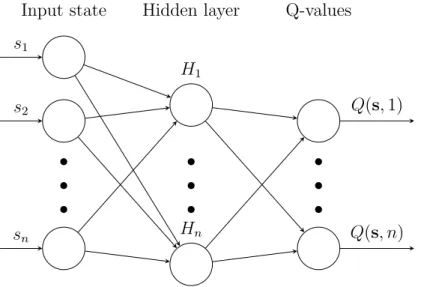
Q-learning is very efficient in simple environments with small state and ac-tion spaces but is not suitable for many real world problems with large state spaces (order of thousand and more). For example, if we consider training a RL agent to play famous Atari games and define a state as a single raw pixel map with 200x200=40000 pixels, then given the number of colors is 256 (for grayscale image), number of states in our state space will be equal to 25640000. Such a large state space precludes the use of table-based methods. Furthermore, since for convergence it is required to visit each state-action pair sufficiently many times, it makes such problems computationally intractable because number of episodes required for converges becomes extremely large. In order to deal with these serious issues it was proposed [33] to replace conventional Q-table with neural network or Q-network, a function approxi-mator which inputs state representation as a multidimensional feature vector and outputs Q-values of the different actions for this state (see Figure 3.3).
Training Q-network comes down to minimizing the following loss function:
L= (r+γmax
a Q(s
′
, a)−Q(s, a))2, (3.7) where L – loss function being minimized, r – immediate reward, Q(s, a) – action-value function for the state-action pair (s, a), Q(s′, a) – action-value function for the state-action pair (s′, a), γ – discount factor.
CHAPTER 3. REINFORCEMENT LEARNING FUNDAMENTALS 26
..
.
..
.
..
.
s1 s2 sn H1 Hn Q(s,1) Q(s, n) Input state Hidden layer Q-valuesFigure 3.3: Deep Q-network architecture.
Intuition behind the equation (3.7) is that two adjacent states s′ and s only differ with respect to the discount factor γ and transition (immediate) reward r. Therefore, difference between values of adjacent states should be as small as possible, which is achieved by minimizing the function specified above.
In order to improve the convergence speed and stability of Q-network algorithm, additional measures should also be taken. This includes using experienced replay and freezing target network techniques [33].
Experienced replay is aimed at breaking correlations between adjacent states during the training process and preventing the optimization procedure being trapped into a poor local minimum of the objective function (3.7). The main idea is to store all transitions between states into replay memory in the form of tuple (st, a, st+1, r) and use them later during the training phase. Replay memory is usually large enough to retain several hundred thousands transitions from few hundreds previous episodes. During the training phase, instead of using the most recent transitions, we randomly sample minibatch of transitions from the replay memory and use them for fitting neural network.
Target network freezing implies that the computation of max
a Q(s
′, a) in
(3.7) should be done using separate neural network (“target network”) which is periodically (every several hundred episodes) synchronized with the main neural network whose weights are being constantly adjusted on each iteration. This allows to stabilize computation of the target values max
a Q(s
CHAPTER 3. REINFORCEMENT LEARNING FUNDAMENTALS 27
Algorithm 4 Q-network algorithm with experienced replay and target net-work freezing
Input: initial states, memory M, Qmain, Qtarget,ϵmin,ϵmax, ∆ϵ,
updateIn-terval
Initialize: ep := 0, ϵ:=ϵmax
1: repeat
2: if Rand0to1()<max(ϵ, ϵmin) then
3: a := GetRandomAction(s) 4: else 5: a:= arg max i Qmain(s, ai) 6: end if 7: snext, r :=GetNextState(s)
8: add (s, snext, r, a) to replay memory M
9: sample minibatch (s(i), s(i)
next, r(i), a(i)) from memory M
10: y(i) := { r(i),if s(i) is terminal state r(i)+γmax aQtarget(s (i) next, a(i)),otherwise
11: trainQmain using s(i) as inputs andy(i) as responses
12: if ep % updateInterval == 0 then 13: Qtarget :=Qmain 14: end if 15: ϵ:=max(ϵmin, ϵ−∆ϵ) 16: ep := ep + 1 17: s:=snext 18: until terminated
The classical Q-network algorithm (see Algorithm 4) had been shown to have several drawbacks which were partially eliminated in the more recent studies. In particular, due to the argmax operator used in action selection and target values evaluation, the algorithm tends to deliver too optimistic estimates of Q-values, which can often lead to suboptimal policies. The solu-tion to this problem is proposed in the study [45] which introduces the idea of Double Deep Q-Network (DDQN). DDQN architecture decouples target values computation and the best action selection operations by using two different Q-networks which are updated interchangeably. Another extension is discussed in the research paper [47] and revolves around Dueling Deep Q-Network (Dueling DQN). The core idea of this concept is to split hidden layer into two parts (streams) computing estimates of state values and ac-tions advantages independently. These estimates are then combined by the output layer to produce familiar Q-values. It is interesting to mention that
CHAPTER 3. REINFORCEMENT LEARNING FUNDAMENTALS 28
several advanced Q-network methods, including ones described in the cur-rent section, can be combined into Rainbow algorithm [16] which has been claimed to achieve unprecedented convergence speed and performance in the Atari environment.
3.5
Policy gradient
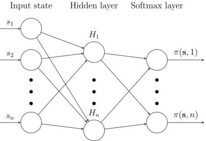
In contrast to Q-network algorithm policy gradient (see Algorithm 5) is not used to approximate Q-table, instead, it learns target policy directly by map-ping input state to the probability distribution of actions (see Figure 3.4).
..
.
..
.
..
.
s1 s2 sn H1 Hn π(s,1) π(s, n) Input state Hidden layer Softmax layerFigure 3.4: Policy network architecture.
According to the policy gradient theorem [41], gradient of any differen-tiable policy can be expressed as
∇w=Eπ{∇logπ(w)(s, a)Q(s, a)}, (3.8)
where ∇w – gradient of weights of the policy network, π(w)(s, a) – policy network which outputs probability of the action a in the state s, Q(s, a) – action-value function for the state-action pair (s, a),Eπ{·}– expectation
un-der the policy π(w).
The closed-form gradient expression (3.8) allows using gradient-based op-timization methods for finding the optimal policy.
In many RL tasks (e.g. Go game) reward only comes upon reaching the terminal state bringing us to the so-called credit assignment problem, one
CHAPTER 3. REINFORCEMENT LEARNING FUNDAMENTALS 29
Algorithm 5 Policy gradient algorithm
Input: initial states, policy network π(w), buffer M repeat
repeat
a:=SampleAction(πw(s))
snext, r := GetNextState(s, a)
add (s, a, r) to the buffer M
s:=snext
untilepisode has finished
(optional) apply variance reduction to the rewards in M
for (s, a, r) in Mdo
w:=w+∇logπ(w)(s, a)r end for
until terminated
of the most fundamental problems in the RL field. This problem reduces to the fact that it is difficult to determine which actions (and to which extent) taken during the episode contributed to achieving this specific reward. Con-sequently, it becomes non-trivial to estimate action-value function Q(s, a) of the state-action pairs visited during the episode. There are at least two ways how to handle this issue. The first and the most naive approach is to treat the finally obtained reward as a sample of the action-value function for all state-action pairs which were observed during the episode. Then for each state-action pair these samples can be averaged over sufficient number of episodes to produce estimates of the action-values function. Practically this often works well, but the convergence speed may decrease dramatically and the finally obtained policy may be suboptimal. The second approach is to try to estimate values Q(s, a) of state-action pairs using separate neural network Qθ(s, a) in parallel with learning action gradients. These estimates Qθ(s, a) will then replace the action-value function Q(s, a) in the gradients
equation (3.8):
∇w=Eπ{∇logπ(w)(s, a)Qθ(s, a)}, (3.9)
where∇w– gradient of weights of the policy network,π(w)(s, a) – policy net-work which outputs probability of action a in the state s, Qθ(s, a) – neural
network with weights θ estimating action-value function for the state-action pair (s, a),Eπ{·}– expectation under the policyπ(w).
CHAPTER 3. REINFORCEMENT LEARNING FUNDAMENTALS 30
for dealing with credit assignment problem and improving learning perfor-mance of the policy gradient. In this case, the actor is a conventional policy gradient performing action selection, whereas the critic is a standard DQN algorithm estimating action-value functionQ(s, a) for each state-action pair. It is worth mentioning that in addition to vanilla policy gradient and actor-critic approach there are several other policy gradient variations fun-damentally different from the classical versions. For example, the study [39] introduces and proves convergence of the deterministic policy gradient which outputs exact action rather than a probability distribution over actions. The study [28] extends this idea to continuous action spaces, which allows using policy gradient in continuous control algorithms. Natural policy gradient [26] is another perspective research direction which takes different view on the gradient computation itself and is claimed to provide promising results.
Chapter 4
Graph signal sampling as
rein-forcement learning problem
In the previous chapters we considered theoretical foundations of machine learning for graph signal recovery as well as RL basics. In this chapter we turn our theoretical knowledge into practice by developing novel algorithms for graph signal sampling. We start our discussion by proposing MAB-based RL algorithm in the Section 4.1 followed by the deep RL algorithm utilizing policy gradient approach in the Section 4.2. Finally, Section 4.3 discusses difficulties associated with usage of RL for graph signal recovery.
4.1
Proposed sampling algorithm based on
the stochastic MAB
The problem of selecting the sampling setMand recovering the entire graph signal x from the signal values x[i] can be interpreted as a RL problem. Indeed, we consider the selection of the nodes to be sampled being carried out by an “agent” which crawls over the empirical graphG. The set of actions our sampling agent may take is A={1, . . . , H}.
A specific action a∈ A refers to the number of hops the sampling agent performs starting at the current node it to reach a new nodeit+1, which will be added to the sampling set, i.e., M:=M ∪ {it+1}. In particular, the new node it+1 is selected uniformly at random among the nodes which belong to its a-step neighbourhood N(it, a) (see Figure 4.1).
The problem of optimally selecting actions at given time can be formu-lated as a MAB problem. Each arm of the bandit is associated with an action. In our setup, a sampling strategy (or policy) amounts to specifying a probability distribution over the individual actions a ∈ A. We parametrize
CHAPTER 4. GRAPH SIGNAL SAMPLING AS RL PROBLEM 32
it
N(it,1) N(it,2) N(it,3)
Figure 4.1: The filled node represents the current location itof the sampling
agent at time t. We also indicate the 1-, 2- and 3-step neighbourhoods.
this probability distribution with a weight vector w = (w1, . . . , wH) ∈ RH
using the softmax rule:
π(w)(a) = e
wa
∑
b∈A
ewb
The weight vector w is tuned in the episodic manner with each episode amounting to selecting sampling set M based on the policy π(w). At each timestep t the agent randomly draws an action at according to the
dis-tribution π(w) and performs transition to the next node i
t+1 which is se-lected uniformly at random from the at-step neighbourhood N(it, at). As
was mentioned earlier, the node tt+1 is added to the sampling set, i.e.,
M:=M ∪ {it+1}. We also record the actionatand add it to the action list,
i.e., L :=L ∪ {at}. The process continues until we obtain a sampling set M
with the prescribed size (sampling budget) M.
Our goal is to learn an optimal policyπ(w)for the sampling agent in order to obtain signal samples which allow recovery of the entire graph signal with minimum error. We assess the quality of the policy using the MSE incurred by the recovered signal ˆxM which is obtained via (2.2) using the sampling set Mby following policy π(w):
R :=− 1
N
∑
j∈V
(x[j]−xˆM[j])2
The obtained reward is associated with all actions/arms which contributed to picking samples into sampling set during the episode. For example, if the sampling set has been obtained by pulling arms 1, 2 and 5, the obtained reward will be associated with all these arms, because we do not know what is the exact contribution of the specific arm to the finally obtained MSE.
CHAPTER 4. GRAPH SIGNAL SAMPLING AS RL PROBLEM 33
The key idea behind gradient MAB is to update weightswso that actions yielding higher rewards become more probable under π(w) [40, Chapter 2.8]. According to the aforementioned book weights update can be accomplished using gradient ascent algorithm:
wa:= { wa+αR(1−π(a)), a=ak wa−αRπ(a),∀a̸=ak for k = 1..M −1, a∈ A, ak∈ L (4.1)
The single difference between update rule (4.1) and one presented in the book [40, Eq. 2.10] is that in our case weights update is performed in the end of each episode and not after an arm pull. That is because we do not know reward immediately after pulling an arm and should wait until the whole sampling set is collected and reward is observed. The intuition behind the update equation (4.1) is that for each arm which has participated in picking a node into sampling set (a =at), the weight is increased, whereas weights
of remaining arms (∀a ̸= at) are decreased. In both cases degree of weight
increase/decrease is scaled by the reward obtained with help of this arm as well as by the learning rate α. For faster convergence in our implementation, instead of stochastic gradient ascent we use mini-batch gradient ascent in combination with RMSprop technique [44] (see Algorithm 6 for implementa-tion details).
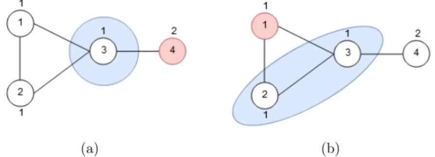
Choice of the gradient MAB algorithm can be additionally justified by the study [5] which shows that in the environments with non-stationary rewards probabilistic MAB policy can result in higher expected reward in comparison to single-best action policies. In our problem non-stationarity of reward arises from the graph structure itself, i.e., reward distribution for a particular arm of a bandit depends on the location of the sampling agent. Suppose sampling budget M is 2 and consider example presented in Figure 4.2. In case (a) sampling agent is initially located at node 4. By pulling arm #1 it can only pick node 3 which is in the other cluster. It is easy to verify that by using recovery method (2.2) graph signal will be perfectly reconstructed (MSE = 0). On the other hand, case (b) shows the situation when the agent can only pick nodes 2 or 3 belonging to the same cluster as currently sampled node, leading to non-zero reconstruction MSE.
The whole process of weight updates is repeated for sufficient number of episodes until convergence is reached and the optimal stochastic policy is attained. Described above learning procedure can be efficiently summarized in the form of pseudocode (see Algorithm 6).
Obtained probability distributionπ(w)represents sampling strategy which incurs the minimum reconstruction MSE when using the convex recovery
CHAPTER 4. GRAPH SIGNAL SAMPLING AS RL PROBLEM 34
Algorithm 6 Online sampling and reconstruction with MAB Input: empirical graph G, sampling budget M, batch size B, α Initialize: w :=0,M={∅},L={∅},∇w=0,g=0, ep= 0
repeat
select starting nodei∈ V randomly
M:={i} L={∅}
for t:= 1;t < M do
a:=SampleAction(π(w))
inext :=SampleNode(G,N(i, a))
M:=M ∪ {inext} L:=AppendToList(L, a) i:=inext end for ˆ x∈arg min ˜ x ∥x˜∥TV
s.t. x[i] =x[i] for all˜ i∈ M
R:=−1 N ∑ j∈V (x[j]−x[j])ˆ 2 for k := 1;k < M do for a:= 1;a⩽H do ∇wa:= { ∇wa+R(1−π(a)), if a=L[k] ∇wa−Rπ(a), otherwise end for end for ep:=ep+ 1 if ep modB = 0 then g:= 0.9g+ 0.1(∇w)2 w:=w+α∇w/√g ∇w:=0 end if
until convergence is reached Output: π(w)
CHAPTER 4. GRAPH SIGNAL SAMPLING AS RL PROBLEM 35
(a) (b)
Figure 4.2: Illustration of reward being conditioned on the position of a sampling agent. In this picture: red node – current position of the sampling agent, blue region – nodes within distance 1 from the sampling agent. Node indices are shown inside the nodes, signal values – outside.
method (2.2).
4.2
Sampling algorithm based on the policy
gradient
In the previous section we presented an algorithm which did not use any notion of state during the learning process. However, this important infor-mation may potentially vastly improve performance of the learning algorithm if a state is chosen appropriately. For instance, at each time step sampling agent may not simply draw an action from the probability distribution, but also take into account state of the current node which can be a compact feature vector of the node in some way summarizing its place within the graph. The intuition is that the nodes belonging to the same clusters should have similar states which, in turn, should trigger similar actions. On the other hand, the problem of choosing suitable state representation for a node is rather challenging. At the first glance, the most straightforward measure which could be used for defining a state is a local clustering coefficient of a node:
ci =
2|E(N(i))|
ki(ki−1)
,
whereE(N(i)) denotes the set of edges connecting two different neighbors of node i and ki denotes number of neighbors node i has.
Although the measure summaries relationships between neighbors around current node, it is too local to differentiate between different locations of
CHAPTER 4. GRAPH SIGNAL SAMPLING AS RL PROBLEM 36
nodes in the graph.
A 1 B 0.5 D 1 C 0.5 E 0.5 F 1 H 0.5 G 1
Figure 4.3: Using local clustering coefficient as a state (clustering coefficient values are shown outside the nodes).
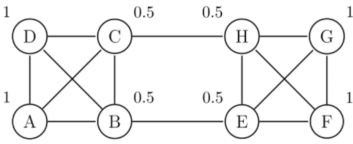
From Figure 4.3 it can be easily noticed that multiple nodes, which are in different clusters, may have the same states/clustering coefficient values (e.g. nodes A and F both have clustering coefficient 1). This makes action selection ambiguous and has a detrimental effect on learning process.
This problem can be overcome if instead of clustering coefficients one would use feature vectors, such as node2vec [13]. Node2vec is an embedding algorithm which utilizes popular in natural language processing word2vec paradigm [11] and matches a node to a feature vector of a predefined length. Consequently, this feature vector can be directly used as an input of the policy gradient algorithm (see Algorithm 7).
It should be noted that the feature selection for graph nodes is a non-trivial process and requires careful consideration. The major obstacle is that the derivation of the feature vectors from the data often requires computa-tionally expensive pre-processing making this approach simply impractical.
4.3
Reward choice problem
Traditionally, reward function occupies central part of any reinforcement learning algorithm and has a direct impact on its convergence and general stability. Usually, in RL applications reward serves as a measure of success and is used to encourage actions yielding higher expected reward. For in-stance, if the goal of an agent is to escape a labyrinth, then the huge reward should be given when the agent accomplishes this task. Similarly, in graph signal sampling the most naive and straightforward measure of success is mean squared error of recovery. Since we aim at achieving the smallest pos-sible reconstruction error, the smaller MSE should lead to the larger reward. This can be accomplished by using negative MSE reward measure, as it was
CHAPTER 4. GRAPH SIGNAL SAMPLING AS RL PROBLEM 37
Algorithm 7 Online sampling and reconstruction with policy gradient Input: empirical graph G, sampling budget M, batch size B
Initialize: w,M:={∅},H:={∅}, ep:= 0 repeat
select starting nodei∈ V randomly
M:={i}
for t:= 1;t < M do
s:=GetState(i)
a:=SampleAction(π(w)(s))
inext :=SampleNode(G,N(i, a))
M:=M ∪ {inext}
add (s,a,reward placeholder) to history buffer H
i:=inext end for ˆ x∈arg min ˜ x ∥x˜∥TV
s.t. x[i] =x[i] for all˜ i∈ M
R:=−1
N
∑
j∈V
(x[j]−x[j])ˆ 2
populate reward placeholders inH with actual reward R ep:=ep+ 1
if ep modB = 0 then for each (s,a,r) in H do
fit policy network π(w) using (s,a,r) end for
clear H
end if
until convergence is reached Output: π(w)
CHAPTER 4. GRAPH SIGNAL SAMPLING AS RL PROBLEM 38
already demonstrated in the previous sections: R :=− 1
N
∑
j∈V
(x[j]−xˆM[j])2
The problem with using the aforementioned reward is that for its cal-culation one should know beforehand true underlying graph signal. This measure is acceptable in such applications as data compression where we al-ready have all the data at our disposal and need to select sampling set which would minimize decoding error. However, in problems related to regression or data reconstruction from only finite number of known measurements us-age of such a reward function is problematic. One possible reward measure which does not rely on true signal values and is available immediately from the graph signal recovery formulation is the objective function of the SLP algorithm:
R :=−min ˜
x ∥x˜∥TV
s.t. x[i] =x[i] for all˜ i∈ M.
(4.2) However, it is disputable what is the relation between optimal value of the SLP and the quality of the recovered graph signal. It may seem natural to assume that since in the SLP we aim at minimizing total variation, we can use negative SLP objective value as a reward (4.2). This assumption may be misleading, because if obtained signal is smooth it may still have huge mean squared error. 1 1 1 2 2 2 (a) 1 1 1 1 1 1 (b)
Figure 4.4: Illustration of clustered graph signal and the result of incorrect recovery (a) – underlying true graph signal and sampled node (shown in black), (b) – recovered graph signal.
Consider the graph signal with two clusters depicted in Figure 4.4. Signal values within each cluster are the same and equal to 1 and 2 respectively. Suppose we sample arbitrary node in the first cluster and try to recover whole graph signal based on it. It is easy to verify that by using familiar SLP procedure one can get perfectly smooth signal with optimization objective
CHAPTER 4. GRAPH SIGNAL SAMPLING AS RL PROBLEM 39
being zero. However, in this case all signal values in the second cluster will be completely incorrect and mean squared error will be non-zero.
In addition to the reward measures described above, another measure that may seem reasonable is Shannon’s entropy. If we define minimum and maximum values of our graph signal asmandM and quantize the signal to a grid withn divisions then the Shannon’s entropy can be calculated according to the following formula:
H=−
n
∑
i=1
Pilog(Pi), (4.3)
where Pi is a probability of graph signal values falling into the interval:
Pi =P rob ( ˆ xM ∈[m+ (M −m)(i−1) n ;m+ (M −m)i n ) ) . (4.4)
Then the reward simply becomes:
R:=H (4.5)
The intuition behind the entropy maximization is that we aim at sampling graph signal in such a way so that the recovered signal carries maximum information or, in the other words, has maximum entropy.
In the Section 5.4 we conduct experiments on the synthetic dataset to understand how Shannon’s entropy as well as objective function of SLP are suitable for being used as reward measures and how they are connected to the MSE of signal recovery.
Chapter 5
Numerical experiments
This chapter describes models used in our simulations, experiments per-formed and results obtained.
5.1
Simulation model
In our experiments we use a synthetic dataset generated in accordance to the stochastic block model (SBM). SBM is a simple probabilistic model for representing graphs which contain communities. Within SBM a graph is partitioned into l clusters with sizes Nl. The probability of having an edge
between nodes of the same cluster is denoted p, whereas the probability of edge between the nodes of different clusters is denoted q. Such a model has been found a particularly useful because it has been extensively studied from many perspectives [10, 15, 34] and allows for a relatively simple theoretical analysis. In addition to the SBM model assumption we make sizes of clusters Nl follow the geometric distribution:
Nl ∼Geometric(s) (5.1)
with probability mass function being
P r(Nl=k) = (1−s)k−1s, k ={1,2,3, ...} (5.2)
The parameter s is known as “probability of success” and ranges from 0 to 1. Formula (5.1) allows generation of clusters with non-uniform sizes (more smaller clusters and fewer larger ones), which enables more consistent imitation of the real-world data.
A simple but useful model for clustered graph signals is: x=∑
C∈F
aCtC, (5.3)
CHAPTER 5. NUMERICAL EXPERIMENTS 41
with the cluster indicator signals tC[i] =
{
1, if i∈ C
0 else.
The partition F underlying the signal model (5.3) can be chosen arbitrarily in principle. However, our methods are expected to be the most useful if the partition matches the intrinsic cluster structure of the empirical graphG. The clustered graph signals of the form (5.3) conform with the network topology, in the sense of having small TV ∥x∥TV, if the underlying partition F =
{C1, . . . ,C|F |}consists of disjoint clusters Cl with small cut-sizes. Relying on
the clustered signal model (5.3), [23, Thm. 3] presents a sufficient condition on the choice of sampling set such that the solution ˆxof (2.2) coincides with the true underlying clustered graph signal of the form (5.3). The condition presented in [23, Thm. 3] suggests choosing the nodes in the sampling set preferably near the boundaries between the different clusters.
5.2
Experiments with MAB-based sampling
algorithm
We now verify the effectiveness of the proposed sampling set selection al-gorithm (Alal-gorithm 6) using synthetic data and compare it to two other existing approaches, i.e., random walk sampling (RWS) and URS discussed earlier in Section 2.2. We define a random graph with 10 clusters where sizes of clusters are drawn from the geometric distribution with probability of suc-cesss = 8/100. In accordance to the SBM intra- and inter-cluster connection probabilities are parametrized asp= 7/10 andq = 1/100. We then generate a clustered graph signal according to (5.3) with the signal coefficients aCl =l for l = 1,2, ...,10. Example of a typical instance of random graph with such parameters is shown in Figure 5.1.
Given the model we generate training data consisting ofK = 500 random graphs and for each graph instance we run Algorithm 6 for 10000 episodes, which is sufficient to reach convergence.
In Figure 5.3 we illustrate the mean policy
π(w) = 1 K K ∑ i=1 πi(w) (5.4)
The finally obtained policy (5.4) is then evaluated by applying it to 500 new i.i.d. realizations of the empirical graph, yielding the sampling setsM(i),
CHAPTER 5. NUMERICAL EXPERIMENTS 42
Figure 5.1: Empirical graph obtained from the stochastic block model with p= 7/10 and q= 1/100.
Figure 5.2: Convergence of gradient MAB for one learning instanceGi
CHAPTER 5. NUMERICAL EXPERIMENTS 43
Figure 5.3: Mean policy for the stochastic block model family G.
Figure 5.4: Test set error obtained from graph signal recovery based on different sampling strategies.
CHAPTER 5. NUMERICAL EXPERIMENTS 44 1 1 1 1 2 2 2 2 3 3 3 3 4 4 4 4
Figure 5.5: Toy model for deep reinforcement learning experiment. Signal values are shown outside of the nodes.
i = 1, . . . ,500, and measuring the normalized mean squared error (NMSE) incurred by graph signal recovery from those sampling sets:
N M SEGi = ∥xˆ(i)−x(i)∥2 2 ∥x(i)∥2 2 N M SE = 1 500 500 ∑ i=1 N M SEGi
We perform similar measurements of the NMSE for random walk and random sampling algorithms under different sampling budgets and convert results to the logarithmic scale (see Figure 5.4).
5.3
Experiments with deep reinforcement
learn-ing
In the Section 4.2 we discussed how policy gradient can be potentially used for graph signal sampling. In this section we generate toy graph (see Figure 5.5) which we use to compare stateful policy gradient sampling against state-less MAB sampling. Moreover, in order to study better the impact of the state space choice on the sampling performance we use two different state representations – feature vector obtained with help of node2vec and local clustering coefficient of a node. As a policy network we use a neural network with one hidden layer and 100 neurons in it. Size of the input layer and, respectively, dimensionality of feature vectors in node2vec algorithm is set to 3. Simulation results obtained over 5000 episodes are shown in Figure 5.6. We also illustrate layout of the features in the node2vec feature space in the Figure 5.7.
CHAPTER 5. NUMERICAL EXPERIMENTS 45 0 1000 2000 3000 4000 5000 Iterations 0.0 0.2 0.4 0.6 0.8 1.0 1.2 1.4 M ea n sq ua re d er ro r MAB
Policy Gradient with node2vec
Policy Gradient with local clustering coefficient
Figure 5.6: Convergence process of the deep RL approaches.
5.4
Experiments with reward choice
In this section we conduct experiments on the applicability of such alterna-tive reward measures as objecalterna-tive function of sparse label propagation and Shannon’s entropy of the recovered signal. We generate a graph conforming to the SBM (p = 0.7, q = 0.02) with 10 clusters each one containing 10 nodes. In each simulation round we sample the graph using URS algorithm and recover it using the convex recovery method (2.2). We then measure mean squared error of graph signal recovery and also note the optimal value of the objective function of the SLP obtained during the current simulation round. This pair of measurements is added to the scatterplot (see Figure 5.8) as one data point. This procedure is repeated for 500 simulation rounds so that the scatterplot accounts for 500 data points in total. We conduct two independent simulations, one with sampling budget M = 10 (see Figure 5.8(a)) and the other with sampling budget M = 20 (see Figure 5.8(b)).
We also perform similar experiment to one described above, but instead of the optimal value of the objective function of the SLP in each simulation round we measure Shannon’s entropy and show it in the scatterplot against the mean squared error of recovery (see Figure 5.9). Again, we do the experi-ment for two sampling budgets, i.e.,M = 10 (see Figure 5.9(a)) andM = 20
CHAPTER 5. NUMERICAL EXPERIMENTS 46 Feature 1 −0.6−0.5 −0.4−0.3 −0.2−0.1 0.0 0.1 0.2 Fe ature 2 −1.00 −0.75−0.50 −0.250.00 0.250.50 Feat ur e 3 0.4 0.6 0.8 1.0 1.2
Figure 5.7: Layout of the features in the feature space. (see Figure 5.9(b)).
CHAPTER 5. NUMERICAL EXPERIMENTS 47
120 140 160 180 200 220 240 260 280 Final value of the sparse label propagation objective
0 2 4 6 8 10 M ea n sq ua re d er ro r of r ec ov er y (a) 75 100 125 150 175 200 225 250 Final value of the sparse label propagation objective 2.5 5.0 7.5 10.0 12.5 15.0 17.5 20.0 M ea n sq ua re d er ro r of r ec ov er y (b)
Figure 5.8: Scatterplot between mean squared error of recovery and optimal value of the SLP optimization objective: (a) – sampling budgetM = 10, (b) – sampling budget M = 20.
CHAPTER 5. NUMERICAL EXPERIMENTS 48 1.0 1.2 1.4 1.6 1.8 2.0 2.2 Shannon entropy 0 1 2 3 4 5 6 7 8 M ea n sq ua re d er ro r of r ec ov er y (a) 0.4 0.6 0.8 1.0 1.2 1.4 1.6 Shanno