Learning with Low-Quality Data: Multi-View Semi-Supervised Learning with Missing Views

(1)

Learning with Low-Quality Data: Multi-View Semi-Supervised Learning with Missing Views By

Brian Quanz

Submitted to the Department of Electrical Engineering and Computer Science and the Faculty of the Graduate School of the University of Kansas

in partial fulfillment of the requirements for the degree of Doctor of Philosophy

Committee members

Luke Huan, Chairperson

Xue-wen Chen Victor Frost Bo Luo Brian Potetz Zsolt Talata Date defended: 7/24/2012

(2)

The Dissertation Committee for Brian Quanz certifies that this is the approved version of the following dissertation :

Learning with Low-Quality Data: Multi-View Semi-Supervised Learning with Missing Views

Luke Huan, Chairperson

(3)

Abstract

The focus of this thesis is on learning approaches for what we call “low-quality data” and in particular data in which only small amounts of labeled target data is available. The first part provides background discussion on low-quality data issues, followed by preliminary study in this area. The remainder of the thesis focuses on a particular scenario: multi-view semi-supervised learning.

Multi-view learning generally refers to the case of learning with data that has multi-ple natural views, or sets of features, associated with it. Multi-view semi-supervised learning methods try to exploit the combination of multiple views along with large amounts of unlabeled data in order to learn better predictive functions when limited labeled data is available.

However, lack of complete view data limits the applicability of multi-view semi-supervised learning to real world data. Commonly, one data view is readily and cheaply available, but additionally views may be costly or only available in some cases. This thesis work aims to make multi-view semi-supervised learning approaches more applicable to real world data specifically by addressing the issue of missing views through both feature generation and active learning, and addressing the issue of model selection for semi-supervised learning with limited labeled data.

This thesis introduces a unified approach for handling missing view data in multi-view semi-supervised learning tasks, which applies to both data with completely missing additional views and data only missing views in some instances. The idea is to learn a feature generation function mapping one view to another with the mapping biased to

(4)

encourage the features generated to be useful for multi-view semi-supervised learning algorithms. The mapping is then used to fill in views as processing. Unlike pre-viously proposed single-view multi-view learning approaches, the proposed approach is able to take advantage of additional view data when available, and for the case of partial view presence is the first feature-generation approach specifically designed to take into account the multi-view semi-supervised learning aspect.

The next component of this thesis is the analysis of an active view completion scenario. In some tasks, it is possible to obtain missing view data for a particular instance, but with some associated cost. Recent work has shown an active selection strategy can be more effective than a random one. In this thesis, a better understanding of active approaches is sought, and it is demonstrated that the effectiveness of an active selection strategy over a random one can depend on the relationship between the views.

Finally, an important component of making multi-view semi-supervised learning ap-plicable to real world data is the task of model selection, an open problem which is often avoided entirely in previous work. For cases of very limited labeled training data the commonly used cross-validation approach can become ineffective. This the-sis introduces a re-training alternative to the method-dependent approaches similar in motivation to cross-validation, that involves generating new training and test data by sampling from the large amount of unlabeled data and estimated conditional probabil-ities for the labels.

The proposed approaches are evaluated on a variety of multi-view semi-supervised learning data sets, and the experimental results demonstrate their efficacy.

(5)

List of Figures

2.1 Three aligned graphs . . . 19

2.2 Regularized similarity graph for 90 samples of synthetic data . . . 23

2.3 Artificial pathways used to generate test data . . . 25

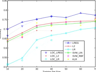
2.4 Average Accuracy vs. Training Set Size for Synthetic Data . . . 31

2.5 Average Accuracy vs. Regularization Parameter for Synthetic Data . . . 32

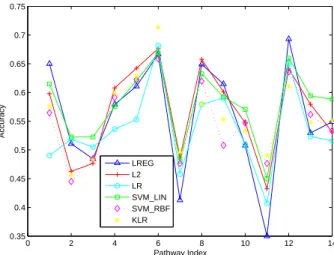
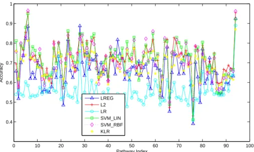
2.6 Average Accuracy vs. Pathway Index for Diabetes Data . . . 33

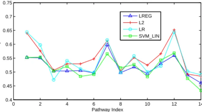
2.7 Average Accuracy vs. Pathway Index for Breast Cancer Data . . . 35

2.8 Average Accuracy vs. Pathway Index for Yeast Data: Partitioning Estimate . . . . 36

2.9 Average Accuracy vs. Pathway Index for Yeast Data: Bootstrap Estimate . . . 36

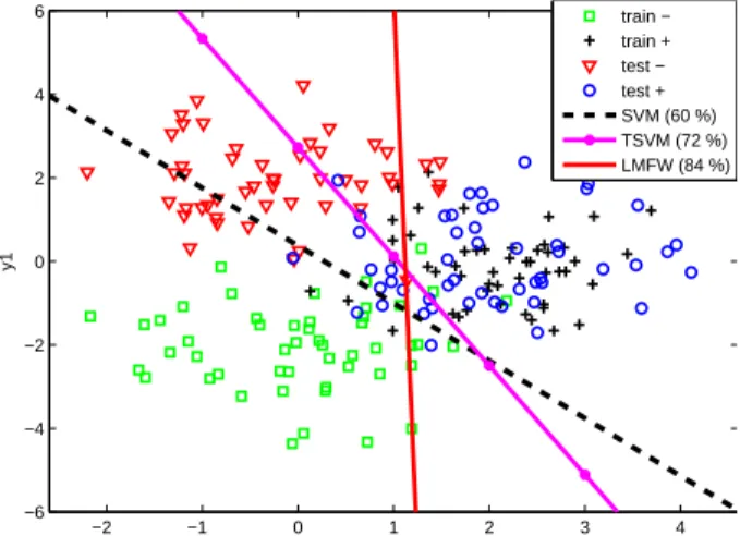
3.1 Decision boundaries for the standard support vector classifier (black) and our method (red) on a simple generated 2-D transfer learning problem. This example is dis-cussed in detail in Section 3.5. . . 40

3.2 Performance of different support vector classifiers on a simple generated 2-D trans-fer learning problem. . . 53

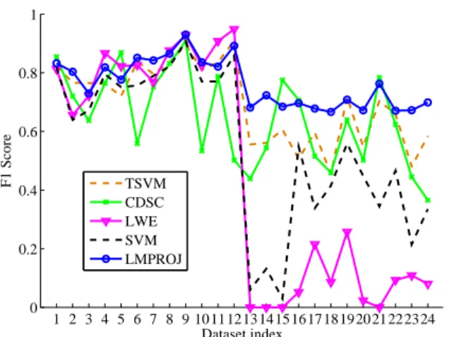
3.3 Prediction F1 score on all 24 data sets . . . 58

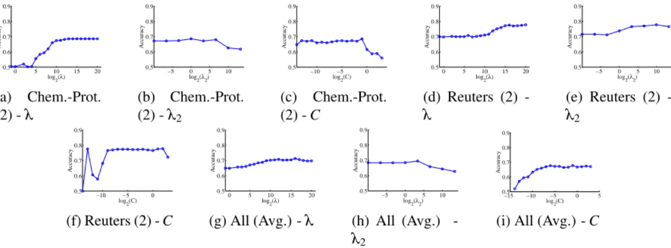
3.4 Parameter Sensitivity . . . 60

4.1 Comparison of features identified from different embedding methods for the Syn-thetic data set 1. . . 79 4.2 Comparison of embeddings found for Synthetic Experiment 2 - see text for details. 81

(13)

4.3 Comparison of embeddings found for Synthetic Experiment 3 . . . 83 4.4 Accuracy vs. num. labeled target data instances . . . 93 4.5 Hyper-parameter sensitivity results - accuracy vs. hyper-parameter settings . . . . 94 6.1 An Example Illustrating View Expansion. . . 110 6.2 Example feature generation network model, where inputs are entered at the bottom

and computations propagate through to the top. . . 112 6.3 Sample of two views of data generated for an ideal 2D test case . . . 119 6.4 Test error vs. mean fraction of view 2 present for the 2-Gaussian data set . . . 119 6.5 Performance criteria vs. contrasting view regularization parameter and vs. number

of hidden units in hidden layer 1 for 0% second view data for the 2-Gaussian data set120 6.6 Test error vs. mean fraction of view 2 present for the WebKB Course data set . . . 123 7.1 Needed differencesq−p∗withr=0.5 andβT≤1 vs.β andT for different values

ofβ orT. . . 140 7.2 Axis-aligned rectangle, sample data generated . . . 144 7.3 Test Accuracy vs. Iteration for 3 selection strategies on the synthetic data set,

averaged over 500 random trials . . . 145 7.4 Test error and MCC vs. iteration for the different selection strategies on the Course

data set, modified Course data set, and Citeseer data set, averaged over 100 random trials . . . 149 7.5 Test error vs. iteration for active selection for varying top fractions of data to

choose select from, on the Course data set, modified Course data set, and Citeseer data set, averaged over 100 random trials . . . 150 8.1 Sample of two views of data generated for 2D test case . . . 164 8.2 Ground truth and estimated test error (z-axis) vs pairs of hyper-parameters for

(14)

List of Tables

2.1 Estimated related pathways found with global test (p-value<0.1) for the Diabetes

data set . . . 28

2.2 Results on synthetic test data for aligned graph classification methods . . . 30

2.3 Pairedt-test results on synthetic test data across 100 iterations, between each pair of methods. A positive 1 indicates the method in the row performed significantly better on average than the method in the column, a negative 1, worse, and a 0 that the difference in performance of the two methods was not statistically significant according to thet-test at the 5% level. . . 30

2.4 Results on diabetes data for aligned graph classification methods for the Insulin Signaling Pathway . . . 34

2.5 Pairedt-test results on diabetes test data across 30 iterations, between each pair of methods. A positive 1 indicates the method in the row performed significantly better on average than the method in the column, a negative 1, worse, and a 0 that the difference in performance of the two methods was not statistically significant according to thet-test at the 5% level. . . 34

3.1 Accuracies for All Methods on Text Classification Datasets . . . 60

3.2 Accuracies for All Methods on Protein-Chemical Datasets . . . 60

3.3 Break down of data sets . . . 62

(15)

4.2 Mean and std. dev. of accuracy out of 100 runs for each method on EPA data set, for increasing amounts of labeled target data . . . 91 4.3 Mean and std. dev. of specificity out of 100 runs for each method on EPA data set 92 4.4 Mean and std. dev. of sensitivity out of 100 runs for each method on EPA data set . 92 4.5 Comparison with state-of-the-art, mean and std. dev. of accuracy out of 100 runs

for increasing amounts of labeled target data . . . 93 4.6 Results when incorporating additional source data features, mean and std. dev. of

accuracy out of 100 runs for increasing amounts of labeled target data . . . 95 6.1 Mean±std. dev. of test error from 200 trials for each method on the 2-Gaussian

data, for 0% second view data available. . . 120 6.2 Mean±std. dev. of MCC from 100 trials for each method on the WebKB Course

data, for varying amounts of average second view data available in fraction of all data instances. Comparison for the case of using pre-training and both the view-matching and contrasting view components (“CoNet”) with neither compo-nent (“No Reg.”), just the view-matching compocompo-nent (“VMR Only”) and just the contrasting view component (“CVR Only”). The first half, “fill” corresponds to filling in cases with available view 2 data, i.e., using whatever view 2 data is avail-able and “no fill” to using only the generated view 2 data. . . 124 6.3 Mean±std. dev. of MCC, F1 score, and test error from 100 trials for each method

on the Chemical Toxicity data, for varying amounts of average second view data available in fraction of all data instances. . . 125 6.4 ANOVA multi-comparison test results for each of MCC, F1 score, and test error

criteria on the Chemical Toxicity data, for 0.15 fraction of view 2 data present. A “1” indicates significant difference in mean between the two methods at the 5 percent level. . . 126

(16)

6.5 Mean±std. dev. of MCC, F1 score, and test error from 100 trials for the CoNet method on the chemical toxicity data. Comparison for the case of using no pre-training and both the view-matching and contrasting view components (“CoNet”) with neither component (“No Reg.”), just the view-matching component (“VMR Only”) and just the contrasting view component (“CVR Only”). The first half, “fill” corresponds to filling in cases with available view 2 data, i.e., using whatever view 2 data is available and “no fill” to using only the generated view 2 data. . . . 126 8.1 Data sets, characteristics, and multi-view semi-supervised learning algorithm used. 164 8.2 Model selection methods used. . . 170 8.3 Mean±std. dev. of MCC, F1 score, and test error over 100 trials for each data set

for the different model selection approaches, with best scores shown in bold. The data sets are ordered by increasing amount of labeled data. . . 172 8.4 Significance testing results at the 5 percent level for paired t-tests between the

proposed approach, SDS, and other model selection approaches for MCC on the Citeseer data set and test error on the rest. A “1” indicates a significant difference in means, “0” not significant, and a “+” indicates SDS did better, “-” worse. . . 172 8.5 Significance testing results at the 5 percent level for paired t-tests between the

rank sum combined approach, SDS+ADA, and other model selection approaches for MCC on the Citeseer data set and test error on the rest. A “1” indicates a significant difference in means, “0” not significant, and a “+” indicates SDS+ADA did better, “-” worse. . . 173 8.6 Significance testing results at the 5 percent level for paired t-tests between SDS

using label outputs, SDS-L, and other model selection approaches for MCC on the Citeseer data set and test error on the rest. A “1” indicates a significant difference in means, “0” not significant, and a “+” indicates SDS-L did better, “-” worse. . . 173

(17)

Chapter 1

Introduction

In data mining or machine learning, a fundamental goal is to be able to predict some quantity of in-terest about some data based on computational representations of the data with measurable features for each instance of the data. For instance we might want to predict the categories present in an image such as "car" or "fish" based on features of the image such as texture or shape descriptors or whether or not a certain chemical has a toxic (carcinogenic) effect in humans based on its chemical structure and in-vitro lab tests. Data mining and machine learning methods try to look at collected sets of data called training data, e.g., images or chemicals, that are annotated with ground truth, or “label”, information about some property of interest for each data instance, e.g., image category or toxicity, in order to estimate, or learn, the relationship between the representations of the data and the labels. In an ideal scenario, collected data ishigh-quality. That is an abundant amount of labeled data is fully available, all from the target data source of interest. In the ideal high-quality data case, labeled data is abundant - so that predictors can be estimated with high confidence, the labeled data is all from the same fixed source as the data for the target task, all the features of the data are available in all instances, data instances are independent, and there are no erroneous data or outliers - extreme values not representative of the data which can mislead learning algorithms. Unfortunately, such ideal high-quality data scenarios are rarely encountered in real-world appli-cations due to error, difficulty, and cost associated with collecting and annotating data. Typically

(18)

data have one or more of the following low-quality aspects.

∙ Only a small sample of labeled data is available from the target data.

∙ The data is only partially observed - i.e., there are missing values.

∙ There are errors, outliers, or noise present in the data and annotations.

∙ The distribution of the target data is not the same as the distribution of the training data, so that the relationships learned in the collected data may not be accurate for the target data. This includes such issues as concept drift where the target data distribution changes over time, and sample selection bias where the collected data sample is not representative of the target data sample.

The focus of this thesis is on the first case, of limited labeled data. It is often the case that only a limited amount of labeled data can be collected for new tasks, due to such factors as time and cost. When labeled data is limited, it becomes more important to make use of any additional sources of information available - which can be in the form of different but related sets of data that are fully labeled, different representations of the data (sets of data features), information about the relationships between features of the data, and unlabeled data from the target data source. In general, the type of low-quality issues along with the specific form of auxiliary information available, whether data or some type of prior knowledge, determines the specific learning problem. For instance when little or no labeled data is available from the target data distribution, but a different set of high-quality labeled data is available from a related distribution, it may be desirable to make use of this data in learning a predictive model for the target data, in some sense transferring knowledge from one task to a related one. This corresponds to both issues of limited labeled data and differing data distributions. The same issue arises if the data are unavoidably different, as is the case with concept drift. Both of these cases correspond to the problem oftransfer learning[142], and the auxiliary information available comes in the form of the related high-quality data. My previous work in this area focused on how to learn a predictive model using related but different

(19)

training data along with unlabeled target data that could then be applied to the target data [148], and also how to find an embedding for training and target data that would align the data distributions and ideally remove the low-quality aspects from the data as a type of pre-processing [149, 150]. Another line of my previous work with limited labeled data is on utilizing auxiliary information in the form of a known relationship between features of the data [147, 66]. These works are discussed chronologically in the first part (the next three chapters) of this thesis, comprising preliminary study on learning with low-quality data, and learning with limited labeled data in particular.

The main focus of this thesis, multi-view semi-supervised learning, corresponds to a different learning problem for the case of small amounts of labeled training data. There are two key types of auxiliary information associated with multi-view semi-supervised learning. The first corresponds to prior knowledge about the features of the data - in the form of a natural partition of the fea-tures, such that each partitioned set is sufficient for learning (as explained in Section 1.2) and also such that the views are not entirely dependent on each other so that some different information is potentially available. The second corresponds to the semi-supervised learning aspect, learning when an additional, usually large, set of unlabeled data is available. This thesis can be seen as also addressing an additional low-quality data aspect often associated with multi-view semi-supervised learning in real world applications - that of structured missing values in the form of missing views. That is, some data instances may be completely missing additional views of the data.

The remainder of this chapter proceeds as follows. First, more detail and background are provided in Sections 1.1 and 1.2. Next, the motivation behind the main focus of this thesis is described in Section 1.3. In Section 1.4, the contributions of this thesis are described. In the last section, Section 1.5, the organization for the remainder of the thesis is given.

1.1

Supervised and Semi-Supervised Learning

The general goal of machine learning is to learn a predictive function f :X →Y mapping an input data space X to an output label spaceY using a set of training data examples. The

(20)

char-acteristics of the label space for a learning problem determine the corresponding machine learning task, for instance if Y is fixed and finite the task corresponds to classification and if Y ≡_ℝ

the task corresponds to regression. Supervised learning addresses the case where a training data set consists of a set of data and label pairs, (x1,y1),(x2,y2), . . . ,(xn,yn)∈X ×Y . In order to

employ supervised learning, data must be collected and annotated with labels, usually by a hu-man. In many scenarios, unlabeled data examples are abundant but obtaining labeled data for a target learning task can be error-prone, time-consuming, expensive, or even impossible. Semi-supervised learning approaches aim to make use of the available unlabeled data to improve the predictive performance of the learned function, particularly in cases where the amount of labeled training data is small. Specifically, in addition to the training examples, a set of unlabeled training instances, xn+1,xn+2, . . . ,xn+m∈X, is available. While the unlabeled data alone do not provide

any information about the predictive function mapping, the combination of the unlabeled data, specific assumptions about the data, and the limited labeled data can make it possible to learn a function with improved predictive performance compared to a function learned using only the limited labeled training data [224]. Typically this improvement is possible through a reduction in some sense of the size of the hypothesis space for the predictive function [224]. A main category of semi-supervised learning methods, and the focus of this thesis, is multi-view semi-supervised learning.

1.2

Multi-View Learning and Multi-View Semi-Supervised

Learn-ing

Multi-view learning generally addresses the case of learning with data that has multiple natural views, generally corresponding to distinct sets of features, associated with it. Specificallyx∈X

can be naturally represented as x= (x1,x2, . . . ,xk)∈X1_×_X2_×_{. . .}_×_Xk_{, corresponding to} _k

different views of the data. For example, when classifying webpages, two natural views for a given webpage could be considered: the set of text features for any text on the webpage, and the

(21)

set of link text features for any links to the webpage. Another example is chemical data. The set of chemical structure features could correspond to one view and chemical-protein interaction profiles could correspond to a second view. Multi-view semi-supervised learning methods try to exploit the combination of multiple views with associated assumptions along with large amounts of unlabeled data in order to learn better predictive functions when limited labeled data is available. The fundamental idea exploited for multi-view semi-supervised learning is the idea of predictive function agreement (consensus) of view-specific functions’ predictions on the unlabeled data. If for each view a function from an associated hypothesis class exists that can achieve zero prediction error, restricted to that view, then all of these functions from different views must agree exactly in their predictions on all data instances, in particular the unlabeled data instances. Therefore, when learning the predictive functions for the views, any combination of functions that disagree in their predictions on the unlabeled data can be eliminated from consideration. In this way, the size of the set of hypothesis functions that explain the labeled data well in each view can potentially be reduced. In the more realistic case that the best performing functions in each view have some base error, as long as the error is not too great there will still necessarily be overlap between these functions’ predictions even if they do not universally agree on all instances [58]. In this case the solutions can still be biased toward predictors that mostly agree on the unlabeled data instances. The condition that for each individual view there exists an associated function from a given hypothesis class that is able to achieve the best possible error rate is referred to asview sufficiency.

1.3

Motivation

Multi-view data arises naturally in many applications. However, lack of complete view data limits the applicability of multi-view semi-supervised learning to real world data. A common scenario is that one data view is readily and cheaply available, but additional views may only be available in some cases and may be costly to obtain.

(22)

This proposed work aims to make multi-view semi-supervised learning approaches more ap-plicable to real world data specifically by addressing the issue of missing views.

1.3.1

Some Motivating Examples

The following are some detailed examples of potential applications that fit the multi-view semi-supervised learning scenario, with missing views being an issue.

1.3.1.1 Medical Diagnostics

In terms of medical diagnosis, in particular cancer diagnosis, prognosis prediction both before and after treatments can be cast as a multi-view semi-supervised learning problem. For instance, if the goal is survival prediction, since the data is censored ground truth labels are not obtainable for many patients. If the goal is to determine pathologic complete response, potentially invasive surgical procedures are required which furthermore are not entirely accurate, making ground truth labels difficult to obtain. Additional views for patients can be obtained but these can be both costly and inconvenient for the patients. For disease diagnosis in general, in many cases there is no definitive test for a disease, or the disease can only be determined with more certainty after many expensive tests such as ultrasound, MRI, and biopsy or after analyzing the results of different treatments. For instance, a common test for elevated thyroid stimulating hormone levels could indicate hypothyroidism, a pituitary adenoma, or a number of auto-immune diseases, with no reliable single test to determine the underlying cause. Obtaining all sets of views for all patients is prohibitively costly and in some case impossible, as is the case with obtaining label information. Ideally, a diagnostic system could aid doctors by considering all partial view information available and including undiagnosed patient information. This problem also motivates an active solution where expensive and invasive procedures are only carried out if necessary. On the other hand, there are some common sets of easily obtainable clinical features which would correspond to a view present for all patients related to a particular disease. For instance, for lung cancer, common clinical factors include forced expiratory volume, performance status, and gender.

(23)

Recently an active multi-view semi-supervised learning approach was applied to data for long cancer survival prediction and pathologic complete response prediction for chemo-radiotherapy treatment, with promising results [209]. In these experiments, additional views were provided for individual patients by imaging techniques like PET/CT scanning.

1.3.1.2 Cheminformatics

For prediction tasks involving chemicals, molecular structure features based on chemical graphs can be readily obtained, but obtaining chemical-protein interaction profiles for a set of proteins can be costly and time-consuming. Other expensive or difficult to obtain views include general in-vitro tests and bio-assay screening, and various more complete characterizations of structure, such as the results of nuclear magnetic resonance and x-ray crystallography. Additionally, labels are also difficult to obtain, particularly when the goal is to evaluate new chemical compounds, for the purpose of drug discovery and evaluation. If the final goal is to predict whether or not a chemical would make an effective and safe drug, the amount of labeled data is limited. Another goal is to determine side effects for a chemical compound, since so few drugs make it to the clinical trial phase there is only a limited amount of data available about the side effects of drugs. Another example is with chemical toxicity prediction, an earlier step in the drug discovery process. In this case, reliable end-points are usually determined using animal studies which are both expensive and time-consuming, and also not entirely accurate.

A small set of complete data has been used with multi-view semi-supervised learning for ad-verse drug effect predictions [54], but for new chemicals or chemical groups additional views will generally not be readily available.

1.3.1.3 Webpage Data

Webpage data potentially contain many views, which may or may not be present in a given in-stance, including images, sounds, and information about incoming links. A standard view that is always present is the text on the webpage itself. Additionally, classifying webpages manually

(24)

would involve hiring human annotators; the process would be time consuming and expensive, and error-prone due both to human error and the ambiguity of assigning a class to a webpage in some cases. Furthermore, new classification tasks are constantly arising as the result of user-specific preferences and search. For instance, a user’s particular preferences about what kind of webpages he or she likes and also what webpages are relevant to a particular semantic search correspond to prediction tasks with little to no labeled instances. More generally, this idea applies to personalized prediction of other kinds as well, for instance such as for personalized product recommendation.

Considering in particular the additional view associated with the text of links on other pages linking to a given webpage, the availability of this view is also limited. As an example, the WebKB data presented in the first work on co-training [25] and used in subsequent work [220, 210] uses text features for text on a webpage as one view, and text features from the incoming link text as a second view. This second view is actually incomplete even in the WebKB data set, but the incomplete view instances are just removed for the purposes of the experiments. For instance, for the faculty vs. student classification task, about half of the webpages in each category do not have any incoming links. However it is likely other pages do link to these, just that the crawler used to collect the webpages did not find them in its finite search. Additionally, as new webpages are created initially no incoming link information will be available, and existing webpages being updated also changes this information; this may lead to misleading representation in the link view if the same procedure is used for generating this view.

1.3.1.4 Multimedia Data

Another category of examples is with media data, for example, tagged and annotated multi-media data such as tagged images. In this case the annotation or tagging can be sporadic and noisy, in the sense that tags may not necessarily correspond to categories present in media or desired categories. Taking tagged images as an example, when available, tags may provide highly relevant information as to the categories of objects or concepts captured in an image, but as annotators cannot be obtained to annotate every image or new images, ideally it would be preferable to be

(25)

able to use tag information when available to improve a classifier for the single image view. Ad-ditionally new classification tasks are likely to arise, limiting the amount of labeled data available in such cases, for instance, as with webpage classification for each user there may be multiple new classification tasks defined, characterizing a particular type of image he or she is looking for based on high-level concepts.

1.3.2

Motivation from Theoretical Work

In order to determine what kind of bias to assert when trying to estimate missing views, a key motivation for this thesis comes from theoretical study of multi-view semi-supervised learning. As mentioned in Section 1.2, if each view is sufficient then multi-view semi-supervised learning may offer some benefit, but another condition is necessary to determine whether or not it will offer a benefit. Theoretical work characterizing what conditions are sufficient for multi-view semi-supervised learning to succeed in improving predictive performance is a key motivation for the proposed approach of this thesis for handling missing view data, and discussed in more detail in Chapter 6. In short, conditions of expansion [9], and differences in empirical kernel maps using the unlabeled data [179] are connected in characterizing how the labeled and unlabeled data are related to each other in different views. These works motivate the idea of this thesis of using the difference between the distance profiles with respect to the unlabeled data in each view for determining if pairs of views provide sufficiently complementary information when evaluating candidate values for filling in missing views, and for estimating the utility of completing an instance for active view completion. This motivates the feature generation (Chapter 6) and active view completion (Chapter 7) approaches of this thesis work.

1.4

Contributions

This analysis of the commonality of theoretical results on multi-view semi-supervised learning leads to the first proposed contribution of this thesis: a novel way of biasing the values selected

(26)

for missing views so that the filled in values will be useful for multi-view semi-supervised learn-ing algorithms. A unified approach for handllearn-ing misslearn-ing view data in multi-view semi-supervised learning tasks is introduced, which applies to the complete range of missing view data. The idea is to use the criteria for the success of multi-view semi-supervised learning algorithms to bias a fea-ture generation function mapping one view to another. This is carried out using additional terms in the objective function of a feature generation network model that encourages the data instances in distinct views to be nearby different unlabeled instances, and also takes into account classification performance for the generated data. The proposed approach can be seen as a pre-processing step that fills in missing views, and so allows a user’s choice of multi-view semi-supervised learning al-gorithms to be applied to the completed multi-view data. Unlike previously proposed single-view multi-view learning approaches, the proposed approach is able to take advantage of additional view data when available, and for the case of partial view presence is the first feature-generation approach specifically designed to take into account the multi-view semi-supervised learning aspect. The second contribution of my thesis is the analysis of the active view completion scenario, which can be an alternative approach for semi-supervised learning depending on the application. In some tasks, it is possible to obtain missing view data for a particular instance, but with some associated cost, for example, an annotator could be hired to label an image, or a PET/CT scan could be ordered for a patient. Recent work has shown for some data that an active selection strategy can result in faster predictive performance improvement than when instances are randomly selected for view completion [209]. However this work does not consider at all when an active strategy may or may not be useful, and additionally the methods proposed for active selection are not directly applicable to multi-view semi-supervised learning methods in general, as they require, for example, estimates of predictive variance. In this thesis, different selection strategies are analyzed and it will be demonstrated that the effectiveness of an active selection strategy over a random one can depend greatly on the relationship between the views. Additionally a simple active selection approach is proposed for which improved performance is demonstrated in the experimental study. The final contribution of this thesis is on model selection for semi-supervised learning

(27)

algo-rithms with limited labeled data. An important component of making multi-view semi-supervised learning applicable to real world data is the task of model selection, which is often avoided entirely in previous work and excluded from consideration. For cases of very limited labeled training data such as those commonly encountered with multi-view semi-supervised learning scenarios, model selection is a significant challenge, and listed as a key open problem in a recent survey [78]. With missing views this task potentially becomes even more difficult since additional hyper-parameters may need to be selected for the pre-processing step. Experimental results have demonstrated the benefit of multi-view semi-supervised learning in cases of very limited labeled training data (e.g., [220, 25, 179]), but in order for such results to be achievable in practice, some practical method of selecting the hyper-parameters for these methods is necessary. The widely used cross-validation approach can become ineffective with too few labeled training instances [176], and the majority of other proposed model selection methods are specific to the corresponding proposed algorithms and frameworks. For instance one such approach is a marginal likelihood approach, in which hyper-parameter estimation is achieved by numerical procedures attempting to approximately integrate out the model parameters from a particular Bayesian probabilistic model for multi-view semi-supervised learning, and maximizing this marginal likelihood with respect to the hyper-parameters [209] (also called type II maximum likelihood or evidence-based approach). However this requires assuming a particular probabilistic model for the different components of the model and the data, so there is no straight-forward way to apply this approach to, for instance, the iterative co-training algorithm (described in Chapter 5) that may, for example, use a decision tree classifier for one view and a support-vector machine for the other, and whose final output is the result of iterative pseudo-labeling and re-training. Furthermore an approach such as cross-validation allows perfor-mance results to be estimated from actual observed perforperfor-mance of implemented algorithms as opposed to analytic approximations. Therefore my thesis introduces an alternative, a sampling ap-proach similar in motivation to cross-validation in order to estimate model performance. The pro-posed approach involves generating new training and test data by sampling from the large amount of unlabeled data and estimated conditional probabilities for the labels, and like cross-validation

(28)

evaluates performance by re-training models and computing average predicted test errors.

Each component of the thesis is evaluated on several synthetic and real world data sets and the experimental results demonstrate the efficacy of the proposed methods.

1.5

Thesis Organization

The chapters of this thesis together form a cohesive body of work/study on learning with low-quality data and in particular learning with limited labeled data, and multi-view semi-supervised learning with missing views. However the chapters are intended to be independent. While the chapters are related, they were written, and the associated work was carried out, so that each chapter could stand by itself.

The outline of the remainder of this thesis is as follows. First, preliminary study on learning with low-quality data is given in the following three chapters. The first part, Chapter 2, is on work on incorporating the structured relationship between features in learning for limited labeled data problems [147], the second part, Chapter 3, is on adapting a large margin learning algorithm for transductive transfer learning [148], and the final part of the preliminary study, Chapter 4, is on feature extraction for knowledge transfer [150].

Afterwards, a general overview is given of the related work in multi-view semi-supervised learning in Chapter 5. Then Chapters 6, 7, and 8 provide additional background information, details on the proposed methods, and detailed experimental study for the proposed methods of view completion via feature generation, active view completion, and model selection, respectively. Finally, conclusions and key areas of future work drawn from the results of this thesis work are discussed in the final chapter, Chapter 9.

(29)

Chapter 2

Preliminary Study I: Laplacian

Regularization for Structured Input

2.1

Introduction

Consider a p-dimensional multivariate random variableX = (x1,x2, . . . ,xp)∈ℝpwhere there are

some known relationships for the features inX. We investigate the problem of performing effective supervised learning to build accurate classification models for mapping such random variables to class labels, based on observed samples and the relation of the features.

Data with intrinsic feature relationships are becoming abundant in many application domains such as bioinformatics, sensor networks, and social networks among others. For instance, in pathway-based microarray classification, a biological network contains a set of genes, taking val-ues based on their expression levels, and there is a known binary relation of genes: the pathway topology [119, 144]. In this case the goal of the data analysis is to use the expression data to predict a measurable outcome, such as the presence or absence of a disease. In sensor networks, there has been a burgeoning interest in incorporating sensors in everyday life to monitor the environment, supply information, and ensure security. At a given time point regarding the state of the full sen-sor network, the features are the readings of the sensen-sors, and we usually know the topology or the

(30)

physical location of the sensors in relation to each other. The goal of the analysis is to detect events of interest based on the collective values of the sensors in the network.

Exploring the relationship between features is not new. Recently in structured feature selec-tion, supervised learning algorithms have been explored for data sets where features have some natural “structure” relationships [198, 211, 215, 219, 223]. For example, Yuan and Lin explored the situation where features may be naturally partitioned into groups and studied the regression problem of grouped features using a technique called grouped Lasso [211]. Another possible type of structure relationship of features is a hierarchical relation (i.e., a directed acyclic graph defined on features) and that has been explored in [198, 219]. In [215], both group structure and hierarchi-cal relation have been studied in a unified framework. Recently Kim and Xing assumed that all the features fit into a linear chain (e.g., genes in a chromosome) and have studied regression problems for such data sets [109]. All these studies, however, do not consider the general case where a gen-eral undirected graph is defined to capture the structure relationship of features for classification and regression.

Here we extend previous work on structured feature selection and investigate the new classi-fication problem where features of a data set have a natural graph relationship. We assume such relationships are known and fixed among all instances of the data set. We call such a problem an

aligned graph classification problemwhere we may use a graph to model a datum, vertices rep-resent features, edges reprep-resent binary relation between features, and vertex and edge set remains the same across a set of samples. Specifically we formalize our classification problem below.

Problem Statement: the Aligned Graph Classification Problem. Given a random variable

X = (x₁,x₂, . . . ,x_p)∈_ℝp_{, a graph} _G_{is a} _{feature relationship graph}_of _X _{if the vertex set of}_G_is

the p features. Given a set of n observations {(X_i,y_i)}, X_i∈X ⊂_ℝp_, _y

i∈Y ={1,2, . . . ,K},

K ∈_ℕ, i∈[1,n], and a feature relationship graph, the aligned graph classification problemis to build a classification model f :X →Y to assign class labels to unseen random variables inX to minimize expected loss. To simplify discussion, from here on, we restrictY ={1,2}to the binary

(31)

class case, 0-1 loss function (i.e., 1 ify= f(x)and 0 otherwise), and undirected feature relationship graphs. Furthermore, we restrict the feature relationship graph structure to be fixed across the set of observations. In other words, the relationship between features is fixed and thus the edges defined between features are fixed for the aligned graphs, each graph will have the same set of edges but possibly different, but aligned, vertex labels, given by the value the random variable takes for that observation.

One way to perform aligned graph classification is to simply use traditional supervised clas-sification algorithms that do not consider the fixed graph structured represented by the feature relationships. By incorporating the graph structure information along with the vertex labels (fea-ture values) in the classification model construction the aim is to improve predictive performance over methods that only consider the feature values for a given observation. Another approach for aligned graph classification that might be considered is to use graph kernel functions for classifi-cation [86]. Graph kernels map a set of data to a high dimensional Hilbert space without explicitly computing the coordinates of the data. Coupled with kernel machines such as support vector ma-chines, graph kernel methods can be used for tasks include classification [189], regression [51] and feature extraction through principle component analysis [166]. The adoption of existing graph kernels for aligned graphs, however, is not straightforward for two major reasons: (i) most current graph kernels assume discrete node labels and aligned graphs have numeric node labels and (ii) most current graph kernels measure the difference of graph structures while the graph structures do not change in the aligned graph data.

Here instead of exploring graph kernel methods, we adopt the framework of logistic regression and extend the work from numeric data to data with an intrinsic graph structure using regulariza-tion. Logistic regression is a popular statistical method for classification that works by modeling conditional probability distributions using a log-linear model and identifying parameters that max-imize the log likelihood of the data, and has been successfully applied to many problems [84, 120]. Comparing to other classification algorithms, logistic regression has the benefits of probabilistic outputs - the probability of a label is returned as opposed to only a discrete class label - and a

(32)

straight-forward generalization from the binary classification case to the multi-class case. In ad-dition, logistic regression tolerates missing values in data [121]. Many improvements have been proposed and the two most significant ones are (i) adding regularization to the objective func-tion and (ii) applying logistic regression in a kernel space. Incorporating a regularizafunc-tion term that penalizes the square of theL₂ norm of the parameters has been seen to improve the predic-tive performance of the method particularly for high-dimensional and highly-correlated data [34], following the same idea as ridge regression [91] in which, by penalizing theL₂norm of the param-eters, reduced generalization error can be achieved by shrinking the prediction variance at the cost of increasing bias.

Here, we extend theL2 regularized logistic regression with a straight-forward modification of the objective function that allows the model learning to be regularized with respect to the graph structure. The basic idea is to force the parameters to vary smoothly over the graph, the idea being quite similar to recent work in semi-supervised learning. The structure of a similarity graph is incorporated in the learning framework in the form of the Laplacian of the graph; the Laplacian of the graph is used in unsupervised (e.g., [174]) and transductive and semi-supervised learning (e.g., [3, 227] when such a similarity structure exists between the data samples. We pursue a similar idea; to improve prediction we incorporate additional information in the form of the graph structure relating the variables and enforce a smooth parameter variation over the graph structure for the variables by means of regularization. The idea should be of particular interest when less labeled information is available, i.e., for small sample data sets or data sets where the ratio of the number of samples to the dimensionality of the data is small.

In summary, our contributions are

∙ We formalized the aligned graph classification problem for data set where features have a natural structure relationship.

∙ We extended the logistic regression to include the normalized graph Laplacian, incorporating the Laplacian in the regularization term. We showed that this results in a simple modification to the original logistic regression solution and update using the efficient newton-raphson

(33)

approach for finding the zeros of the gradient.

∙ We developed an approach to incorporate the graph Laplacian regularization inkernel logis-tic regression, which uses a basis expansion to allow non-linear functions of the variables, similar to support vector machines.

∙ We performed a comprehensive experimental evaluation, showed that Laplacian regularized logistic regression is an effective method for incorporating the graph structure in the predic-tion problem, evaluated these methods on synthetic and real world data sets and compared the performance of the methods to competing methods including support vector machines and unregularized logistic regression.

The rest of this chapter is organized in the following way. Section 2.2 discusses related work. Section 2.3 presents background information and detailed discussion of our algorithms. Section 2.4 presents the experimental study of our algorithms as compared to competing methods. Finally we give a short conclusion and a discussion of the future work.

2.2

Related Work

We use logistic regression as our framework for building classification models for aligned graph classification; logistic regression has also been used extensively for scientific data analysis. For example, sparse logistic regression was proposed to perform gene selection in [173], a partial least squares with penalized logistic regression algorithm was proposed for high-dimensional, small-sample problems in [67], and in [120] logistic regression is used for feature selection. The approach of [173] has been recently improved in [33] using Bayesian regularization, and applied to the problem of cancer classification, and anL₂penalized logistic regression method for classification was proposed in [223].

In bioinformatics research there has recently been much interest in using computational meth-ods to associate groups of genes such as groups defined by biological pathways (graphs) with a

(34)

clinical outcome such as a disease. For example, a statistical method for determining if a group of genes is significantly related to a clinical outcome by calculating a p-value for the group was proposed in [72]. Another statistical test, the Multi-dimensional Cluster Misclassification test (MCM-test), was proposed in [119] for associating pathways with disease outcomes by modeling expression values for a group of genes as fuzzy sets for each outcome and using the membership of the genes in the fuzzy sets to determine significance. For the similar problem of selecting sig-nificant pathways and performing classification, a random forest approach was proposed in [143]. For the problem of detecting gene-gene interaction, anL₂ regularized logistic regression method was proposed in [144].

Our work is different from existing work in that we use a general graph to capture relationship between features. In our method we consider a graph as a manifold and we factor in the graph topology using graph Laplacian as a regularization factor. Hence the key insight is that the con-ditional probability distribution, as evaluated in the logistic regression, varies smoothly along the manifold representing a graph.

2.3

Methodology

2.3.1

Background and Notations.

A graph G is described by a finite set of nodesV and a finite set of edgesE ⊂V×V. In most applications, a graph is labeled, where labels are drawn from a label set λ. A labeling function λ :V∪E →Σassigns labels to nodes and edges. In node-labeled graphs, labels are assigned to

nodes only and infully-labeled graphs, labels are assigned to nodes and edges. Here we consider node labeled graphs only since nodes represent features for a sample.

Following convention, we denote a graph as a quadrupleG= (V,E,Σ,λ)whereV,E,Σ,λ are explained before. We represent a graph with n nodes using its adjacency matrix ξ = (ξi,j)n_i,j=1 whereξi,j=1 if there exists an edge incident on nodesiand jinG, and zero otherwise. We use

(35)

ofG, and upper case calligraphic letters, such asG =G₁,G₂, . . . ,G_n, for a set ofngraphs.

Two graphsG,G′arealignedif there exists a 1-1 mappingϕ:V[G]→V[G′]such that(u,v)∈

E[G]if and only if(ϕ(u),ϕ(v))∈E[G′]. Clearly the aligned relation is (i) reflective, (ii) symmetric, and (iii) transitive and hence an equivalence relation. A group of graphs isalignedif the graphs in the group are pair-wise aligned.

Example 2.3.1. In Figure 2.1 we show three graphs defined on 4 features {x₁,x₂,x₃,x₄} with a star topology. Clearly the three graphs are aligned since they have the same topology. We view each graph as an instance of a 4-dimensional variable X_i= (x_i₁,x_i₂,x_i₃,x_i₄)∈_ℝ4_{, i}_∈_[1_,_3]_{with a}

binary relation defined on the 4 features.

Figure 2.1: Three aligned graphs

2.3.2

Logistic Regression.

Before we introduce regularized logistic regression, we briefly overview basic logistic regression [84]. Logistic regression fits a sigmoid function, P(Y =1∣⃗X =⃗x;⃗β) = 1

1+e−⃗βT⃗x =

e⃗βT⃗x

e⃗βT⃗x₊₁, repre-senting the probability the class label takes value 1 given the data sample has values⃗x and the parameters are⃗β, to the training data, here we use⃗x to denote a data vector with an additional feature value of 1 concatenated to the beginning for convenience (to incorporate the intercept). Using the training data we find the parameters⃗β that best fit the data, and can then use the sigmoid function to map any future data vector to a value in[0,1]. The fitting is achieved by maximizing the

(36)

log-likelihood of the data (which we will denote asℓ(⃗β), as it is a function of the parameters⃗β),

∑N_i₌₁{yilog(P(Y =1∣⃗X =⃗xi;⃗β)) + (1−yi)log(1−P(Y =1∣⃗X =⃗xi;⃗β))}, which can be expressed

as: ℓ(⃗β) = N

∑

i=1 {y_i⃗βT⃗xi−log(1+e ⃗_βT_⃗_x i₎_} _(2.1)

, by setting the gradient, ∂ℓ(⃗β)

∂⃗β =∑

n

i=1{⃗xi(yi−P(Y =1∣⃗X =⃗xi;⃗β))} , equal to⃗0. We then find the zeros using an iterative process, the Newton-Raphson algorithm, which requires taking the second derivative of the log-likelihood. We express the derivative and second derivative of the log-likelihood in matrix form so that the update becomes:

⃗_βnew₌_⃗ βold−(∂ 2_ℓ₍⃗_βold₎ ∂⃗β ∂⃗βT )−1∂ℓ( ⃗_βold₎ ∂⃗β (2.2) which is: ⃗ βnew =⃗βold−(XTW X)−1XT(⃗y−⃗p) (2.3) where⃗pis a column vector withp_i=P(Y=1∣⃗X=⃗x_i;⃗βold), andW=diag(p)∗diag(⃗1−p), where

diag(p)signifies a diagonal matrix with diagonal entriesW_ii=p_iand all other entries set to 0, and

⃗_{1 is a column vector of ones, with dimension}_N_{. With the new beta calculated with equation 2.3,}

the probabilities are recalculated (p andW updated), and the process repeats until convergence, measured by the entries ofW becoming close to 0 or by the change in ⃗β becoming close to 0, using some small threshold value.

Thus for each data vector, we learn a set of parameters⃗β, and can then map each data vector to a probability of class label. We can threshold the output from the logistic regression at 0.5 to obtain the predicted class.

2.3.3

Laplacian-Norm Regularized Logistic Regression.

Here we incorporate graph Laplacian as a regularization term in the logistic regression. Before we talk about regularized logistic regression, we define graph Laplacian and normalized graph

(37)

Laplacian.

For an undirected graphGwith the adjacency matrixξ, theLaplacian LofGis:

L=D−ξ; (2.4)

WhereDis the density matrix ofξ, defined asD= (di,j)ni,j=1where

di,j= ⎧  ⎨  ⎩ ∑n_k=1ξi,k ifi= j 0 otherwise

Thenormalized LaplacianisL =D−12LD− 1 2.

Incorporating the normalized graph Laplacian norm as a regularization term in the logistic regression actually results in a simple modification to the original logistic regression solution. Furthermore, substituting the identity matrix for the normalized Laplacian L results in logistic regression with the ridge penalty (the square of theL₂norm ofβ), since⃗βTI⃗β =⃗βT⃗β.

The new objective function becomes:

g(⃗β) = N

∑

i=1 {yi⃗βT⃗xi−log(1+e ⃗ βT⃗xi₎_{} −}1 2λ ⃗_βT_L_⃗ β (2.5)

The new gradient is given by:

∂g(⃗β) ∂⃗β

=XT(⃗y−⃗p)−λL⃗β (2.6)

The new hessian is given by:

∂2g(⃗β) ∂⃗β ∂⃗βT

=−XTW X−λL (2.7)

(38)

⃗_βnew₌_⃗

βold−(XTW X+λL)−1(XT(⃗y−⃗p)−λL⃗βold) (2.8)

2.3.4

Graph Regularized Kernel Logistic Regression.

Kernel logistic regression works by introducing a basis expansion so that f(⃗x) in P(Y =1∣⃗X =

⃗x;⃗β) = 1

1+e−f(⃗x), previously equal to ⃗β

T_⃗_x _{is now equal to} _α

0+∑N_i=1αiK(⃗x,⃗xi) where K(., .) is a

kernel function implicitly defining a Hilbert space and a feature mapping. In order to keep our Laplacian-regularization framework intact, we define a second method. Since the parameters are translated to the feature space, i.e., from ⃗β varying over the p features (vertices) in the input feature space to⃗α varying over the nfeatures in the kernel space, the original constraints on the graph structure are lost for the parametersα. Thus, in order to include the Laplacian regularization in the kernel space it is necessary to translate the graph structure from the input feature space to the kernel feature space. Essentially we want to define a new weighted graph structure between the n-samples such that the similarity function between two n-samples is regularized by the original graph structure (the original graph Laplacian in our framework). This is a similar idea to semi-supervised learning where we define an underlying similarity graph from the data. Here we want the graph created to impose similarity based on the closeness for matching vertices and the smoothness over the vertices.

In order to derive a similarity graph to regularize the alpha parameters, we estimate a sample similarity function that itself is regularized by the Laplacian of the original graph. We start with an edge of weight 1 between each training sample with the same label, of weight 0 (no edge) otherwise, a rough graph with connections between all samples of the same class. To incorporate the original graph structure, we train a logistic regression model to predict probabilities of link connections that is regularized by the original graph Laplacian. To do this we use a similarity measure (in the form of a Gaussian kernel function) between each pair of aligned vertices in the original graph, and fit a set of logistic regression parameters, using the Laplacian regularization. This translates the binary edge existence function to a weight that is regularized by the original

(39)

graph structure, in effect smoothing the similarity function over the original graph structure. To select the vertex-wise similarity parameter (width of the Gaussian) and the regularization parameter,λ, one option is to perform a cross-validation grid search with the training data, enforc-ing only that the thresholded output correctly predicts the link. In this way, the values can still vary smoothly. However, the number of samples in this case becomes(n2−n)/2 (for ntraining sam-ples), since each pair of training samples becomes a new training sample for the edge prediction function, so performing the multiple iterations with this higher sample size set can be time con-suming. As an alternative, we only perform the logistic regression once by settingσ equal to the standard deviation for each feature and using a highλ value to strongly enforce the regularization term (two times the number of new training samples), avoiding the lengthy grid search process.

In this way we can achieve our goal of creating a new graph structure in the kernel feature space that is still regularized by the original graph structure in the input feature space. Figure 2.2 shows a comparison of the rough, original similarity matrix to the derived similarity matrix for 90 training samples from a synthetic data set. The original structure can still be seen in the regressed similarity matrix (e.g., the cross shape) but this structure is softened (regularized).

(a) Similarity matrix de-termined by class mem-bership

(b) Similarity matrix de-rived from regularized regression

(c) Thresholded regres-sion similarity matrix (at 0.5)

Figure 2.2: Regularized similarity graph for 90 samples of synthetic data

2.3.5

Regularized Local Logistic Regression.

Since the regularized kernel logistic regression method described in the previous section is time-consuming to perform in full, we explore another kernel logistic regression method for learning

(40)

nonlinear class boundaries as an alternative, local logistic regression. The motivation is that often we may desire a model that does not find a global fit to the data, but rather a local fit, similar to the nearest neighbor method and local linear regression method. In this case local logistic regression can be used. Local logistic regression results from a simple modification to the original logistic regression formulation; each sample is weighted by how close it is to the input test sample using some smoothed distance function such as the Gaussian kernel, when the model is fitted. This is described by the following weighting of the likelihood (L) equation: L=∏N_i₌₁P(Y =yi∣⃗X = ⃗x_i;⃗β)γi_{, with} _γ

i =e

−∣∣⃗xi−⃗xt∣∣2

2σ2 for test input⃗x_t, which translates into multiplying each term in the

log-likelihood by its sample weight. The Laplacian regularized version is the same as for regular logistic regression, except for weighting samples in the likelihood term of the objective function. The new update equations result by modifying equations 2.3 and 2.8 so thatWii = piγi and⃗y−⃗p

is scaled by the weights (diag(⃗γ)(⃗y−⃗p)). Here increasing the kernel widthσ results in moving closer to the global solution.

In the subsequent discussion for simplicity, we refer to the logistic regression method as “LR”, the Laplacian-regularized logistic regression method as “LREG”, theL₂norm regularized logistic regression method (withL equal to the identity matrix) as “L2”, the kernel logistic regression as “KLR”. Similarly, we refer to the unregularized local logistic regression method as “LOC_LR”, the the L2 norm regularized local logistic regression method as “LOC_L2” and the Laplacian-regularized local logistic regression method as “LOC_LREG”.

2.4

Experimental Evaluation

2.4.1

Data

2.4.1.1 Synthetic Data.

We generated synthetic test data for an undirected graph with 19 vertices described by the 4 arbi-trary created pathways shown in figures 2.3a - 2.3d, which specify the binary relationships between

(41)

the given variables. For our tests we assume all we know is the existence of a relationship between the variables and form the corresponding undirected graph and 19x19 adjacency matrix. To gener-ate data, the graph class is labeled 1 if at least 2 pathways “produce” (take value) 1, otherwise it is 0. A pathway “produces” 1 if all the node values along any path from a start node (at the left) to an end node of the path are greater than 0.5, otherwise it produces 0. Examples are given in figures 2.3e and 2.3f. We indicate a path with all values greater than 0.5 in Figure 2.3e by small arrows. In Figure 2.3f we show a broken path since node (3) has value 0.3 which is less than 0.5. Thus the pathway in Figure 2.3e “produces” a label 1 and the pathway in Figure 2.3f “produces” a label 0. To generate data we randomly generate values for all the nodes in the range [0,1] and test the graph outcome. We generate 100 samples, and continue replacing samples with label 0 until half have label 1.

(a) Pathway 1 (b) Pathway 2 (c) Pathway 3 (d) Pathway 4

(e) Functioning path-way

(f) Non-functioning pathway

Figure 2.3: Artificial pathways used to generate test data

2.4.1.2 Real World Data.

Next, we consider microarray gene expression data classification: given a set of samples of gene expression values and the associated class labels (e.g., disease or no disease), learn a classification model to predict the label of a test sample using its gene expression values as features. We can view the microarray classification task as an aligned graph classification task by considering the biological pathway structures associated with the genes. Here each pathway related to the outcome of interest is represented by an undirected graph with vertices as genes and edges representing the

(42)

or phosphorylation. To obtain the aligned graph structures for our experiments, we extract pathway graphs from a standard source