Variable Selection in Regression using Multilayer Feedforward Network

Volume 15 | Issue 1 Article 33

5-1-2016

Variable Selection in Regression using Multilayer

Feedforward Network

Tejaswi S. Kamble

Shivaji University, Kolhapur, Maharashtra, India, [email protected]

Dattatraya N. Kashid

Shivaji University, Kolhapur, Maharashtra, India., [email protected]

Follow this and additional works at:http://digitalcommons.wayne.edu/jmasm

Part of theApplied Statistics Commons,Social and Behavioral Sciences Commons, and the

Statistical Theory Commons

Recommended Citation

Kamble, Tejaswi S. and Kashid, Dattatraya N. (2016) "Variable Selection in Regression using Multilayer Feedforward Network,"

Journal of Modern Applied Statistical Methods: Vol. 15 : Iss. 1 , Article 33. DOI: 10.22237/jmasm/1462077120

Cover Page Footnote

We thank the editor and anonymous referees for their valuable suggestions which led to the improvement of this article. First author would like to thank University Grant Commission, New Delhi, INDIA for financial support under Rajiv Gandhi National Fellowship scheme vide letter number F.14-2(SC)/2010(SA-III).

Ms. Kamble is a Junior Research Fellow in the Department of Statistics. Email her at [email protected]. Dr. Kashid is a Professor in the Department of Statistics. Email him at [email protected].

Variable Selection in Regression using

Multilayer Feedforward Network

Tejaswi S. Kamble Shivaji University

Kolhapur, Maharashtra, India

Dattatraya N. Kashid Shivaji University

Kolhapur, Maharashtra, India

The selection of relevant variables in the model is one of the important problems in regression analysis. Recently, a few methods were developed based on a model free approach. A multilayer feedforward neural network model was proposed for developing variable selection in regression. A simulation study and real data were used for evaluating the performance of proposed method in the presence of outliers, and multicollinearity.

Keywords: Subset selection, artificial neural network, multilayer feedforward network, full network model and subset network model.

Introduction

The objective of regression analysis is to predict the future value of response variable for the given values of predictor variables. In the regression model, the inclusion of a large number of predictor variables leads to the problems such as i) decrease in prediction accuracy, and ii) increase in cost of the data collection (Miller, 2002). To improve the prediction accuracy of the regression model, one approach is to retain only a subset of relevant predictor variables in the model, and eliminate the irrelevant predictor variables. The problem of choosing an appropriate relevant set from a large number of predictor variables is called subset selection or variable selection in regression.

In traditional regression analysis, the form of the regression model must be first specified, then fitted to the data. However, if a pre-specified form of the model is itself wrong, another model must be used. Searching for a correct model for the given data becomes difficult when complexity is present in the data. A better alternative approach in the above situation would be to estimate a function or model from the data. Such an approach is called Statistical Learning; Artificial

Neural Network (ANN) and Support Vector Machine (SVM) are statistical learning techniques.

ANNs have recently received a great deal to attention in many fields of study, such as pattern reorganization, marketing research etc. ANN is important because of its potential use in prediction and classification problems. Usually, ANN is used for prediction when form of the regression model is not specified. In this article, ANN is used for selection of relevant predictor variables in the model. Mallows’s Cp (Mallows, 1973) and Sp statistics (Kashid and Kulkarni, 2002),

along with other existing variable selection methods, are suitable under certain assumptions with prior knowledge about the data. When no prior knowledge about the data is available, ANN is an attractive variable selection method (Castellano and Fanelli, 2000), because ANN is a data-based approach. ANN is used in this study for obtaining predicted values of the subset regression model. The criteria Cp and Sp are based on prediction values of subset models. Therefore,

we propose modification in Cp and Sp based on predicted values of the ANN

model.

Mallows’s Cp (Mallows, 1973) is defined by





2 2 p p RSS C n p



   (1)

where p is the number of parameters in the subset regression model with p – 1 regressors, RSSp is the residual sum of squares of the subset model, n is the

number of data points used for fitting the subset regression model, and σ2 _is

replaced by its suitable estimates, usually based on the full model. In this study, the following cases are used.

Case 1

A simulation design proposed by McDonald and Galarneau (1975) is used for introducing multicollinearity in the regressor variables. It is given by





  1 2 2 1 1 , 1, 2, , , 1, 2, , ij ij i J X  



Z 



Z _ i n j J

where Zij are independent standard normal pseudo-random numbers of size n, and

ρ2 _{is the correlation between any two predictor variables. The response variable Y}

1 2 3

1 4 5 0 , 1, 2,...,30

i i i i i

Y   X  X  X 



i

where εi ~ N(0,1). To identify the degree of multicollinearity, the variance

inflation factor (VIF) is used (Montgomery, Peck, and Vining, 2006). For this data, the VIFs for the variables are 339.6, 572.5 and 350.1. These VIFs indicates the presence of severe multicollinearity in the data. We compute the value of the

Cp statistic Cp(M) and report the results in Table 1.

Case 2

Data generated in Case 1 is used, and one outlier is introduced by multiplying the actual Y corresponding to the maximum absolute residual by 25. The value of the response variable Y = 8.2235 is replaced by Y = 205.5878. The value of the Cp

statistic Cp(MO) is computed and reported in Table 1.

Case 3

The following nonlinear regression model is generated using the above

Xi,i = 1,2,3 and εi which are generated in Case 1. The nonlinear regression model

is



1 2 3



exp 1 4 i 5 i 0 i i, 1, 2,...,30 Y   X  X  X 



i

The values of the Cp statistic Cp(NL) are computed for the nonlinear regression

model and reported in Table 1.

Table 1. Values of Cp(M), Cp(MO), and Cp(NL).

Regressors in subset model P Cp(M) Cp(MO) Cp(NL)

X1 2 1.8617 3.0077 2.0726 X2 2 2.2565 2.2510 1.0605 X3 2 3.2585 1.9152 2.3498 X1X2 3 2.2237 2.8740 2.0059 X1X3 3 3.8518 3.2340 3.8492 X2X3 3 4.1730 3.4448 3.0179 X1X2X3 4 4.0000 4.0000 4.0000

As seen in Table 1, the criterion Cp selects the wrong subset models for all

the above-cited cases. The statistic fails to select the correct model in the presence of a) multicollinearity alone, b) both multicollinearity and outlier, and c)

nonlinear regression, because OLS estimation does not perform well in each case. Consequently, variable selection methods based on OLS estimator fail to select the correct model.

Regression Model and Neural Network Model

In general, the regression model is defined as



,



f X

 

Y   (2)

where f is any function of predictor variables X1, X2, …, Xk−1 and unknown

regression coefficients β. If f is a non-linear function, then regression parameters are estimated by using nonlinear least squares method (or some other method). If f

is linear, the regression model can be expressed as

 

Y X  (3)

where Y is an n × 1 vector of response variables, X is a matrix of order n × k with 1’s in the first column, β is a k × 1 vector of regression coefficients and ε is an

n × 1 vector of random errors which are independent and identically distributed

N(0,σ2_{I). The least squares estimator of β is given by (Montgomery et al., 2006)}





1

ˆ 

 

X X X Y

 

The predicted value of the regression model is obtained by the fitted equation

ˆ ˆ _

Y X

The prediction accuracy of the regression model depends on the selection of an appropriate model, which means the form of the function (f) must be specified before the regression analysis. If form of the model is not known, then one of the most appropriate alternative methods to handle this situation is artificial neural network.

Multilayer Feedforward Network (MFN)

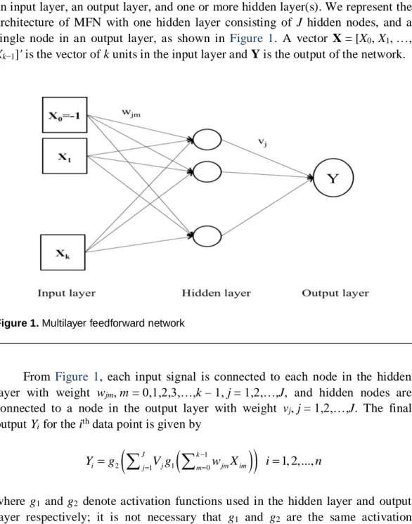
The MFN can approximate any measurable function to any desired degree of accuracy (Hornik, Stinchcombe, and White, 1989). This MFN model consists of an input layer, an output layer, and one or more hidden layer(s). We represent the architecture of MFN with one hidden layer consisting of J hidden nodes, and a single node in an output layer, as shown in Figure 1. A vector X = [X0, X1, …,

Xk−1]' is the vector of k units in the input layer and Y is the output of the network.

Figure 1. Multilayer feedforward network

From Figure 1, each input signal is connected to each node in the hidden layer with weight wjm, m = 0,1,2,3,…,k – 1, j = 1,2,…,J, and hidden nodes are

connected to a node in the output layer with weight vj, j = 1,2,…,J. The final

output Yi for the ith data point is given by







1



2 ₁ 1 ₀ 1, 2,..., J k i _j j _m jm im Y g



_V g



_ w X i n

where g1 and g2 denote activation functions used in the hidden layer and output

layer respectively; it is not necessary that g1 and g2 are the same activation



,



f X



Y  (4)

where β = (v1, …, vJ, w0, w1, w2, …, wk−1), wm = (w1m, w2m, …, wJm),

m = 0,1,2,…,k – 1 and f(X,β) is a nonlinear function of the inputs X0, X1, X2, …, Xk−1 and the weight vector β. If we add an error term in the above

model (4), then it becomes a regression model as in Equation 2, where ε is the random error.

The next step in ANN modeling is training the network. The purpose of training the network is to obtain weights in a neural network model using the training data. Various training methods or algorithms are available in the literature. The robust back-propagation method (see Kasko, 1992) is one such. First, two types of MFN models must be defined, namely the full MFN model and the subset MFN model, for proposing modification in Cp and Sp statistics.

Full MFN and subset MFN model

A full MFN model is constructed with input units X1, X2, …, Xk−1 and bias node

X0 = −1. The MFN model in Equation 4 is a full MFN model. The network

weights are obtained by training the network and the network output vector based on a full MFN model, as

 

ˆ ˆ _{ f X,}

Y  (5)

where ˆ is the estimated weight vector.

A subset MFN model is constructed with a subset of input units

XA = (X0, X1, X2, …, Xp−1)' of size p(p ≤ k) in the input layer. The subset network

model is given by



_A, _A



f X



Y  (6)

where X and β are partitioned as X = [XA : XB] and β = [βA : βB]. Similarly, the

network output vector based on subset MFN model is



ˆ



ˆ _, A A f X  Y  (7)

To implement the training procedure using network training algorithm, we need to select the number of hidden layers in the MFN and the number of hidden nodes in that hidden layer. This is discussed in the next section.

Selection of Hidden Layer and Hidden Nodes

The selection of learning rate parameter, initial weights and number of hidden layers in the MFN model and the number of hidden nodes in each hidden layer is an important task. The number of hidden layers is determined first. The network begins as a one-hidden-layer network (Lawrence, 1994). If the one-hidden-layer MFN network does not sufficient for training the network, then more hidden layers are added. In the MFN model, theoretically a single hidden layer is sufficient, because any continuous function defined on a compact set in Rn _{can be}

approximated by a multilayer ANN with one hidden layer with sigmoid activation function (Cybenko, 1989). Based on this result, we consider the single hidden layer MFN model with sigmoid activation function.

The choice of number of hidden neurons in the hidden layer is also a considerable problem, and it depends on the data. Research has proposed various methods for selection of hidden nodes in the hidden layer (see Chang-Xue, Zhi-Guang and Kusiak, 2005), as follows:

 H1 = 2I + 1 (Hecht-Nelson, 1987)

 H2 = (I + O)/2 (Lawrence and Fredrickson, 1998)

 n/10 − I – O ≤ H3 ≤ n/2 − I – O (Lawrence and Fredrickson, 1998)

 H4 = Ilog2n (Marchandani and Cao, 1989)

 H5 = O(I + 1) (Lipmann, 1987)

Here, I is the number of inputs, O is the number of output neurons, and n is the number of training data points.

Variable Selection Methods and Proposed Methods

In the classical linear regression, several variable selection procedures have been suggested by the researchers. Most methods are based on least squares (LS) parameter estimation procedure. The variable selection methods based on LS estimates of β fail to select the correct subset model in the presence of outlier, multicollinearity, or nonlinear relationship between Y and X. Here, we modified existing subset selection methods using MFN model for prediction.

It is demonstrated that the Mallows’s Cp statistic does not work well when

assumptions are violated. Researchers have suggested some other methods for variable selection (see Ronchetti and Staudte, 1994; Sommer and Huggins, 1996). Also Kashid and Kulkarni (2002) have suggested a more general criterion, the Sp

statistic for variable selection in cases of clean and outlier data. It can be defined as





2

_

_

1 2 ˆ ˆ 2 n ik ip i p Y Y S k p    



  (8)

where Yˆ_ik is the predicted value of the full model, Yˆ_ip is the predicted value of the subset model based on M-estimator of the regression parameters, and k and p are the number of parameters in the full and subset model respectively. The σ2 _is

replaced by its suitable estimates, which usually consists of the full model.

The subset selection procedure is same for both the methods. The Sp statistic is

equivalent to the Cp statistic when LS method is used for estimating regression

coefficients. The following suggests modification in both criteria using the complicity measure.

MCp and MSp Criteria

In a modified version of the Cp and Sp statistics, the network output (estimated

values of response Y) is obtained by using the single hidden layer with a single output MFN model.

The network outputs Yˆ_ik  f

 

X_i,ˆ and Yˆ_ip  f



X_iA,ˆ_A



denote outputs based on full MFN and subset MFN model, respectively. The residual sum of squares for the full and subset network models are defined as









2 1 2 1 ˆ _{, and} ˆ n k i i ik n p _i i ip RSS Y Y RSS Y Y      





The modified version of Cp and Sp are denoted as MCp and MSp. They are defined





2 , , and p p RSS MC C n p



  (9)





2

_

_

1 2 ˆ ˆ , n ik ip i p Y Y MS C n p    



 (10)

where n is the number of data points and p is the number of inputs including bias node (Xo). Yˆ_ik and Yˆip are the predicted values of Y based on the full and subset

MFN models, respectively, C(n,p) is the penalty term, and σ2 _{is replaced by its}

suitable estimate if it is unknown. The motivation for proposing modified versions of Cp and Sp are as follows.

In criterion MCp, we use two types of measures. The first term measures the

discrepancy between the desired output and network output based on the subset MFN model. The smaller this value is, the closer to the desired output it is; the smallest value of this measure is smallest for the full model. Therefore, it is difficult to select the correct model by minimizing criterion. So, we add a complicity measure called the penalty function, comprised of only p, only n, or both n and p.

In the second criterion MSp, we use sum of squared difference between

network output of the full and subset MFN models. The smallest value indicates that a prediction based on the subset MFN model is as accurate as the full MFN model. When full MFN model is itself the correct model, this value is zero. It is difficult to select the correct model using the minimizing criterion. Therefore we added the penalty function similar to criterion defined in (9) and used the same logic for the selection of subset. The selection procedure for both methods is as follows.

Step I: Compute the MCp for all possible subsets.

Step II: Select the subset corresponding to the minimum value of MCp.

Use the same procedure for MSp.

Choice of Estimator of σ2

An estimator of σ2 _{is required to implement the MC}

p and MSp criteria. In the

literature of regression, various estimators of σ2 _{are available. What follows are}

estimators of σ2 _{used in MC}

p and MSp based on full network output, and a study of

1.





2 1 2 1 ˆ ˆ n i ik i Y Y n k  _   



2.



ˆ22 



1.4826median rimedian

 

ri



2 3. ˆ32 



1.4826median ri



2

where n is the number of data points, k is the number of inputs in the full MFN model including bias node r_i  Y_i Yˆ_ik, and Yˆ_ik is the network output for the ith

data point based on the full MFN model.

Performances of MCp and MSp

To evaluate the performance of MCp and MSp, we have used single hidden layer

MFN model and robust back-propagation training method with sigmoid activation function in the hidden layer and output layer. In robust back -propagation, we use an error suppressor function s(e) by replacing the scalar squared error e (Kasko, 1992), because s(e) = e2 _{is not robust. The following error suppressor functions}

are used in this study.

1. E1 = s(e) = max(−c, min(c,e)) (Huber function)

(where c = 1.345 is bending constant)

2. E2 = s(e) = 2e/(1+e2) (Cauchy function)

3. E2 = s(e) = tanh(e/2) (Hyperbolic tangent function)

The learning rate parameter (η) is selected by trial and error, and the number of hidden nodes in hidden layer is selected using the selection methods given earlier. The following seven penalty functions are used for computing MSp and

MCp; some are available in the literature (Sakate and Kashid, 2014).

2. P₂  plog



n2



3. ₃ 2 2



1



2



2 p p P p n p       4. P4  p



logn1



5. ₅ 2 1 pn P n p    6. ₆ 2 2



1



1 p p P p n p      7. P₇  plogn

The performance of the proposed methods is measured for different combinations of penalty functions (Pl)l = 1,2,…,7, selection methods of hidden

nodes in the hidden layer (Hm)m = 1,2,…,5, and error suppressor functions

(Eo)o = 1,2,3; these are denoted by (Pl, Hm, Eo). Three simulation designs are used

for the evaluation of the performance of MSp and MCp.

Simulation Design A

The performance of proposed modified versions of Sp(MSp) and Cp(MCp) are

evaluated using the following models with two error distributions. Model I: Y = β0 + β1X1 + β2X2 + β3X3 + ε, where β = (1,5,10,0),

Model II: Y = β0 + β1X1 + β2X2 + β3X3 + β4X4 + ε, where β = (1,5,10,0,0)

The regressor variables were generated from U(0,1) and the error term was generated from N(0,1) and Laplace (0,1). The response variable Y was generated using Models I and II for sample sizes 20 and 30, respectively. This experiment is repeated 100 times and ability of these methods to select the correct model is measured using learning parameter (η) = 0.1 and 2

1 ˆ

 . The results are reported in Tables 2 through 5.

Table 2. Model selection ability of MSp and MCp in 100 replications for Model I of size 20 Error distribution Error suppressor function H1 H2 H3 H4 H5 Pn MSp MCp MSp MCp MSp MCp MSp MCp MSp MCp Normal Huber P1 79 66 84 77 72 75 73 64 77 71 P2 86 81 92 82 81 87 84 77 87 84 P3 88 86 94 90 90 92 89 86 93 89 P4 88 85 94 88 88 90 87 81 90 87 P5 86 81 92 85 82 87 85 79 88 85 P6 86 81 92 85 82 87 85 79 88 85 P7 85 79 92 82 79 87 82 77 87 84 Cauchy P1 78 58 77 32 76 52 67 57 63 69 P2 91 71 85 35 83 72 79 68 80 76 P3 93 79 85 34 86 77 87 80 84 83 P4 92 74 85 36 84 77 84 74 83 81 P5 91 71 85 36 83 72 79 69 82 76 P6 91 71 85 36 83 72 79 69 82 76 P7 91 70 85 35 82 72 79 66 79 75 Hyperbolic Tangent P1 79 66 74 77 75 79 75 79 77 83 P2 86 81 86 84 85 87 85 87 86 91 P3 88 86 91 89 87 90 87 90 92 91 P4 88 85 88 86 86 89 86 89 89 91 P5 86 81 86 84 85 88 85 88 87 91 P6 86 81 86 84 85 88 85 88 87 91 P7 85 79 85 84 85 87 85 87 85 91 Laplace Huber P1 69 67 75 66 75 69 77 34 78 66 P2 83 81 86 80 87 73 89 36 79 79 P3 86 86 91 84 89 80 94 35 80 81 P4 87 83 88 82 89 76 93 36 81 81 P5 84 81 86 80 87 73 91 36 80 79 P6 84 81 86 80 87 73 91 36 80 79 P7 81 81 86 77 85 73 88 35 79 79 Cauchy P1 74 54 77 52 68 67 70 51 71 62 P2 83 75 81 60 80 77 80 66 78 74 P3 86 85 86 67 84 80 85 76 80 81 P4 86 84 84 65 82 79 84 72 79 78 P5 84 77 82 60 80 77 82 67 78 74 P6 84 77 82 60 80 77 82 67 78 74 P7 83 74 80 60 79 77 79 65 75 73 Hyperbolic Tangent P1 70 67 76 69 85 76 85 76 82 63 P2 83 81 82 82 90 85 90 85 88 75 P3 86 86 87 88 92 89 92 89 93 75 P4 87 84 86 87 92 88 92 88 93 78 P5 84 81 83 83 90 85 90 85 88 76 P6 84 81 83 83 90 85 90 85 88 76 P7 82 81 82 82 90 84 90 84 87 74

Table 3. Model selection ability of MSp and MCp in 100 replications for Model I of size 30 Error distribution Error suppressor function H1 H2 H3 H4 H5 Pn MSp MCp MSp MCp MSp MCp MSp MCp MSp MCp Normal Huber P1 78 72 78 74 71 69 76 62 74 72 P2 89 81 89 88 83 85 90 74 90 92 P3 93 87 92 92 92 87 94 96 92 94 P4 88 77 84 84 78 82 92 72 85 80 P5 87 77 82 82 77 79 92 66 80 79 P6 87 77 82 82 77 79 92 66 80 78 P7 89 81 88 88 83 85 90 74 88 92 Cauchy P1 72 59 74 71 77 59 76 52 70 50 P2 85 73 81 88 84 74 86 68 86 76 P3 94 82 87 93 88 81 94 80 94 80 P4 80 66 83 83 83 69 84 62 80 68 P5 79 65 82 79 81 68 84 60 80 66 P6 79 65 82 79 81 68 84 61 80 66 P7 84 73 81 88 84 74 86 68 86 68 Hyperbolic Tangent P1 83 74 82 71 78 74 74 62 78 76 P2 89 82 93 88 92 87 82 72 90 88 P3 94 87 96 92 94 91 86 68 96 92 P4 85 81 91 81 88 83 86 72 84 83 P5 85 81 88 79 86 82 82 70 85 82 P6 85 81 88 79 86 82 82 71 84 82 P7 88 92 93 88 91 86 82 74 90 86 Laplace Huber P1 73 56 77 70 72 54 80 58 78 62 P2 82 75 91 85 91 80 80 78 88 80 P3 89 81 92 87 90 84 86 86 90 86 P4 82 70 85 81 82 75 81 70 90 76 P5 81 66 84 77 82 72 81 64 91 72 P6 81 66 84 77 82 73 81 65 84 72 P7 82 74 91 85 88 80 80 72 88 80 Cauchy P1 62 33 74 47 77 66 76 56 77 60 P2 78 43 83 66 86 78 86 66 85 76 P3 87 58 87 73 90 80 92 80 87 84 P4 75 40 81 58 84 77 80 62 84 70 P5 73 38 80 56 82 75 78 62 84 66 P6 73 38 80 56 82 75 78 62 84 66 P7 77 43 83 64 86 78 86 66 84 74 Hyperbolic Tangent P1 72 77 72 71 78 68 78 60 82 50 P2 85 90 89 84 85 86 82 78 96 76 P3 88 93 91 89 90 88 86 86 97 84 P4 82 87 84 83 84 83 78 78 94 70 P5 82 86 83 80 82 80 78 78 94 62 P6 82 86 83 80 82 80 78 78 94 62 P7 84 90 89 84 85 87 80 80 98 76

Table 4. Model selection ability of MSp and MCp in 100 replications for Model II of size 20 Error distribution Error suppressor function H1 H2 H3 H4 H5 Pn MSp MCp MSp MCp MSp MCp MSp MCp MSp MCp Normal Huber P1 60 33 60 43 62 50 62 38 68 60 P2 79 53 77 59 72 72 76 60 74 72 P3 85 68 83 78 82 82 85 72 78 85 P4 82 64 83 65 83 78 80 78 76 80 P5 80 57 79 60 72 74 76 64 74 76 P6 80 57 79 60 72 74 76 64 74 76 P7 77 53 76 59 72 70 76 58 74 72 Cauchy P1 54 40 51 24 60 22 48 32 60 43 P2 68 40 72 46 70 38 76 49 70 56 P3 72 43 80 68 82 50 80 56 76 65 P4 71 45 75 64 80 46 80 52 76 63 P5 69 51 73 46 70 38 78 49 78 58 P6 69 63 73 46 70 38 78 49 78 58 P7 66 50 71 42 68 38 74 49 70 56 Hyperbolic Tangent P1 63 42 69 60 50 50 61 44 68 70 P2 74 72 78 72 68 74 88 65 84 84 P3 82 85 82 78 74 82 88 78 94 86 P4 79 83 82 74 74 78 88 78 90 86 P5 75 76 78 74 70 78 88 78 89 85 P6 75 76 79 74 70 76 88 68 88 84 P7 72 70 79 74 66 70 89 68 80 84 Laplace Huber P1 40 44 54 32 56 35 68 48 41 40 P2 62 58 68 52 67 56 76 72 62 60 P3 76 66 88 78 74 75 74 65 70 74 P4 70 65 72 63 76 73 82 76 64 70 P5 65 59 68 52 66 60 76 72 60 60 P6 65 59 68 52 66 60 76 72 61 60 P7 58 58 67 50 66 54 76 70 60 56 Cauchy P1 59 29 50 32 52 32 44 22 44 49 P2 61 40 64 48 74 50 56 45 64 62 P3 64 53 65 56 78 60 58 53 73 72 P4 65 50 64 52 76 58 56 52 67 68 P5 64 43 65 48 74 50 56 48 64 64 P6 64 43 65 48 75 50 56 48 64 64 P7 61 40 62 44 75 46 54 43 62 58 Hyperbolic Tangent P1 54 44 58 44 56 35 52 38 60 60 P2 78 60 78 70 67 57 60 53 74 72 P3 74 66 84 76 74 74 61 56 87 81 P4 74 66 83 76 78 76 62 54 83 80 P5 72 60 78 70 66 60 61 52 74 74 P6 72 60 78 70 66 60 61 52 74 74 P7 70 60 78 78 66 54 61 50 72 76

Table 5. Model selection ability of MSp and MCp in 100 replications for Model II of size 30 Error distribution Error suppressor function H1 H2 H3 H4 H5 Pn MSp MCp MSp MCp MSp MCp MSp MCp MSp MCp Normal Huber P1 69 36 64 55 64 30 72 46 66 46 P2 82 77 83 64 76 60 84 70 84 66 P3 83 87 86 73 78 80 86 76 84 88 P4 80 66 80 63 76 43 82 64 80 64 P5 78 85 72 60 74 40 78 60 78 62 P6 78 58 72 61 74 39 78 60 77 62 P7 83 77 82 64 75 60 84 70 80 66 Cauchy P1 45 25 51 44 52 30 52 23 44 34 P2 68 58 65 68 71 60 72 40 62 52 P3 79 68 74 74 78 66 79 58 78 62 P4 56 51 64 64 68 44 66 32 54 42 P5 57 38 64 64 66 45 65 30 46 42 P6 57 38 64 64 66 44 64 30 46 42 P7 66 54 64 68 70 58 65 40 62 52 Hyperbolic Tangent P1 68 36 70 57 52 53 72 44 56 35 P2 82 76 80 78 70 69 84 72 76 62 P3 82 86 80 86 80 82 86 76 86 80 P4 80 66 78 72 70 74 81 64 68 52 P5 76 60 76 68 66 69 80 62 68 48 P6 76 60 76 69 66 69 79 62 68 48 P7 82 76 81 76 70 69 84 70 32 63 Laplace Huber P1 56 36 54 48 52 56 48 52 52 36 P2 86 50 72 70 74 84 70 74 76 70 P3 92 54 78 74 84 92 74 80 84 70 P4 74 46 66 64 69 80 66 72 70 50 P5 74 46 64 64 62 70 64 72 66 46 P6 74 46 63 64 62 70 64 72 66 46 P7 86 50 72 68 74 84 68 74 76 70 Cauchy P1 32 36 60 24 50 34 40 21 36 21 P2 52 60 80 42 60 62 74 45 56 48 P3 64 74 86 48 74 70 84 56 64 60 P4 40 54 68 32 52 54 62 32 45 36 P5 40 52 66 30 50 48 56 28 42 32 P6 40 52 66 31 50 48 56 28 42 33 P7 48 60 80 40 61 62 72 42 42 42 Hyperbolic Tangent P1 66 44 52 46 50 81 60 46 52 36 P2 80 72 80 66 72 68 81 70 79 64 P3 84 80 84 79 76 80 86 79 86 82 P4 74 66 71 62 74 68 81 66 60 56 P5 72 30 64 56 72 68 75 62 60 48 P6 72 61 64 56 72 68 76 62 60 48 P7 80 70 76 66 72 68 83 70 74 74

From Tables 2 through 5, it can be observed that the overall performance of the

MSp statistic is better than the MCp statistic. The performance of penalties P2

through P7 is better than penalty P1, with H1 through H5, for Models I and II.

Based on these simulations, it is recommended that any hidden node selection method be used with penalty P2 through P7 and Huber or Hyperbolic Tangent

Simulation Design B

The experiment was repeated 100 times using the simulation design A. The performance of MSp and MCp were compared with Mallows’s Cp for Models I and

II with sample sizes of 20 and 30. MSp and MCp were computed using (P3,H1,E1),

and learning parameters (η) = 0.1 and



ˆ

₁2. The results are reported in Table 6.

Table 6. Model selection ability of correct model for 100 repetitions

Error

Distribution Sample sizes

Model I Model II MSp MCp Cp MSp MCp Cp Normal 20 94 90 82 83 78 76 30 92 92 79 86 73 70 Laplace 20 91 84 81 88 78 77 30 92 87 84 78 74 75

From Table 6, it is clear that the model selection ability of MSp and MCp is better

than Cp (based on LS estimates) for sample sizes 20 and 30 for both error

distributions. The model selection ability of MSp is uniformly larger than that of

MCp or Cp.

Simulation Design C

Three further models based on MFN are used to evaluate the performance of MSp

and MCp: Model III: 2 2 2 2 0 1 1 2 2 3 3 4 4 Y    X  X  X  X  , Model IV:

Y

 

 

_{0 1}

X

₁2





₂

X

₂2





₃

X

₃2





₄

X

₄2





, Model V: 2 2 2 2 0 1 1X 2X2 3 3X 4X4

Y



e

    





, where β = (1,5,10,0,0).

In this simulation, Xi = (i = 1,2,3,4) were generated from U(0,1) and error

was generated from N(0,1) and Laplace(0,1). The response variable Y was generated using Models III, IV and V. MSp and MCp were computed using (P1 –

P7,H1,E1), learning parameters (η) = 0.1 and 2 1

ˆ



. The ability of these methods to select the correct model over 100 replications is reported in Table 7.

Table 7. Correct model selection ability over 100 replications

Model III Model IV Model V Error distribution n = 20 n = 30 n = 20 n = 30 n = 20 n = 30 Pn MSp MCp MSp MCp MSp MCp MSp MCp MSp MCp MSp MCp Normal P1 50 40 78 25 71 57 89 65 04 07 72 76 P2 55 35 89 48 78 70 91 73 05 06 90 91 P3 55 24 93 58 83 78 88 60 04 07 90 95 P4 60 38 80 34 80 76 82 56 05 07 91 85 P5 54 37 77 32 79 72 83 56 05 07 83 82 P6 55 40 77 35 79 72 85 65 05 06 89 82 P7 54 34 90 42 76 69 90 70 05 06 75 90 Laplace P1 20 16 60 40 15 16 89 70 07 05 89 19 P2 21 14 80 66 12 14 93 80 07 04 99 18 P3 25 15 86 80 7 11 82 65 06 04 100 13 P4 22 14 75 56 12 15 80 52 05 03 96 10 P5 20 14 75 50 13 16 80 52 05 04 90 16 P6 20 15 75 50 13 16 90 70 08 05 90 16 P7 18 14 80 64 13 14 91 72 04 06 99 14

From Table 7, it is clear that performance of MSp is better than MCp for all models

and sample size 30. The performance of both criteria MSp and MCp is very poor

for all models when error distribution is Laplace for small samples: the sample size must be moderate to large for selection of relevant variables when regression model is nonlinear.

Performance of MCp and MSp in the presence of multicolinearity and

outlier

The performance of MSp and MCp is studied using the Hald data (Montgomery et.

al, 2006). The variance inflation factors (VIF) corresponding to each term are 38.5, 254.4, 46.9, and 282.5. The VIF values indicate that multicollinearity exists in the data. Consider the following cases:

Case I: Data with multicolinearity (original data)

Case II: Data with multicolinearity and single outlier (Y6 = 109.2 is

replaced by 150)

Case III: Data with multicolinearity and two outliers (Y2 = 73.4 and

MSp and MCp was computed for all possible subset models with different

penalty functions and estimators of σ2_{. The selected subset model, by various}

combinations of (Pl,



ˆ

_s2), l = 1,2,...,7, s = 1,2,3 is reported in Table 8. For training

the network, the simulation employs the Huber error suppressor function, number of hidden neurons H1, and learning parameter (η) = 0.1. The results are reported in

Table 8.

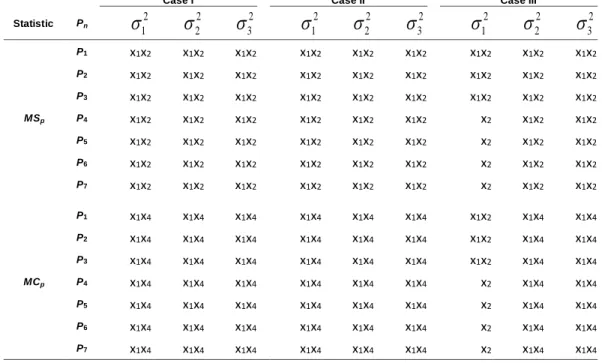
Table 8. Selected subset by MSp and MCp for Cases I – III

Case I Case II Case III Statistic Pn 2 1





₂2



₃2



₁2



₂2



₃2



₁2



₂2



₃2 MSp P1 _{x1x2 x1x2 x1x2 x1x2 x1x2 x1x2 x1x2 x1x2 x1x2} P2 _x1x2 x1x2 x1x2 x1x2 x1x2 x1x2 x1x2 x1x2 x1x2 P3 _x1x2 x1x2 x1x2 x1x2 x1x2 x1x2 x1x2 x1x2 x1x2 P4 _x1x2 x1x2 x1x2 x1x2 x1x2 x1x2 x2 x1x2 x1x2 P5 _x1x2 x1x2 x1x2 x1x2 x1x2 x1x2 x2 x1x2 x1x2 P6 _x1x2 x1x2 x1x2 x1x2 x1x2 x1x2 x2 x1x2 x1x2 P7 _x1x2 x1x2 x1x2 x1x2 x1x2 x1x2 x2 x1x2 x1x2 MCp P1 _x1x4 x1x4 x1x4 x1x4 x1x4 x1x4 x1x2 x1x4 x1x4 P2 _x1x4 x1x4 x1x4 x1x4 x1x4 x1x4 x1x2 x1x4 x1x4 P3 _{x1x4 x1x4 x1x4 x1x4 x1x4 x1x4 x1x2 x1x4 x1x4} P4 _x1x4 x1x4 x1x4 x1x4 x1x4 x1x4 x2 x1x4 x1x4 P5 _x1x4 x1x4 x1x4 x1x4 x1x4 x1x4 x2 x1x4 x1x4 P6 _x1x4 x1x4 x1x4 x1x4 x1x4 x1x4 x2 x1x4 x1x4 P7 _x1x4 x1x4 x1x4 x1x4 x1x4 x1x4 x2 x1x4 x1x4

This data is analyzed in the connection of multicolinearity and outlier ( see

Ronchetti and Staudte, 1994; Sommer and Huggins, 1996; and Kashid and Kulkarni, 2002). They have suggested {X1, X2} is the best subset model for clean

data and outlier data. The MSp statistic selects the same subset model for all

combinations of (Pl,



ˆ

_s2), l = 1,2,...,7, s = 1,2,3, for Case I and II. In Case III, MSp

fails to select correct model for penalty P4 – P7 with 2 1

ˆ



. Conclusion: the MSp

statistic performs better than MCp for all cases with all penalty functions and

Conclusion

The proposed modified methods are model-free. It is clear that the performance of proposed MSp statistic is better than classical regression methods in the presence

of multicollinearity, outlier, or both simultaneously. The MSp statistic selects the

correct model in cases of nonlinear model for moderate to large sample sizes. From the simulation study, it can be observed that MFN is useful when there is no idea about the functional relationship between response and predictor variables. The MSp statistic is also useful for selection of inputs from a large set of inputs in

a network model, in order to find which network output is closest to the desired output.

Acknowledgements

This research was partially funded by the University Grant Commission, New Delhi, India, under the Rajiv Gandhi National Fellowship scheme vide letter number F.14-2(SC)/2010(SA-III).

References

Chang-Xue, J. F., Zhi-Guang, Yu. and Kusiak, A. (2006) Selection and validation of predictive regression and neural network models based on designed experiment. IIE Transactions, 38(1), 13-23. doi: 10.1080/07408170500346378

Cybenko, G. (1989) Approximation by superpositions of sigmoidal functions. Mathematics of Control, Signals, and Systems, 2(4), 303-314. doi:

10.1007/BF02551274

Castellano G. and Fanelli A. M. (2000) Variable selection using neural network models. Neurocomputing, 31(1-4), 1-13. doi: 10.1016/S0925-2312(99)00146-0

Hecht-Nelson, R. (1987) Kolmogorov’s mapping neural network existence theorem. In Proceedings of the IEEE International Conference on Neural Networks 111. New York:IEEE Press, pp. 11-14.

Hornik, K., Stinchcombe, M. and White, H. (1989) Multilayer feedforward networks are universal approximators. Neural Networks, 2, 359-366.

Kashid, D. N. and Kulkarni, S. R. (2002) A more general criterion for subset selection in multiple linear regressions. Communication in Statistics–Theory & Method, 31(5), 795-811. doi: 10.1081/STA-120003653

Kasko, B. (1992) Neural networks and fuzzy systems: a dynamic systems approach to machine intelligence. Englewood Cliffs, N.J.: Prentice-Hall, Inc.

Lawrence, J. (1994) Introduction to neural networks: design theory and applications, 6th _{Ed. Nevada City, CA:California Scientific Software.}

Lawrence, J. and Fredrickson, J. (1998) Brain Maker user’s guide and reference manual. Nevada City, CA:California Scientific Software.

Lippmann, R. P. (1987) An introduction to computing with neural nets.

IEEE Acoustics, Speech and Signal Processing Magazine, 4(2), 4–22. doi:

10.1109/MASSP.1987.1165576

Mallows, C. L. (1973) Some comments on Cp. Technometrics, 15(4),

661-675. doi: 10.1080/00401706.1973.10489103

Marchandani, G. and Cao, W. (1989) On hidden nodes for neural nets. IEEE Transactions on Circuits and Systems, 36(5), 661–664. doi: 10.1109/31.31313

McDonald, G. C. and Galarneau, D. I. (1975) A Monte Carlo evaluation of some ridge-type estimators. Journal of the American Statistical Association,

70(350), 407-412. doi: 10.1080/01621459.1975.10479882

Miller, A. J. (2002) Subset selection in regression. London: Chapman and Hall.

Montgomery, D., Peck, E. and Vining, G. (2006) Introduction to linear regression analysis. New York: John Wiley and Sons Inc.

Ronchetti, E. M. and Staudte, R. G. (1994) A robust version of Mallows’s

Cp. Journal of the American Statistical Association,89(426), 550-559. doi:

10.1080/01621459.1994.10476780

Sakate D. M. and Kashid D. N. (2014). A deviance-based criterion for model selection in GLM. Statistics: A Journal of Theoretical and Applied Statistics, 48(1), 34-48. doi: 10.1080/02331888.2012.708035

Sommer S. and Huggins R. M. (1996). Variable selection using the Wald test and a robust Cp. Journal of the Royal Statistical Society C: Applied Statistics,