Hyperspectral image classification via contextual deep learning

R E S E A R C H

Open Access

Hyperspectral image classification via

contextual deep learning

Xiaorui Ma, Jie Geng and Hongyu Wang

Abstract

Because the reliability of feature for every pixel determines the accuracy of classification, it is important to design a specialized feature mining algorithm for hyperspectral image classification. We propose a feature learning algorithm, contextual deep learning, which is extremely effective for hyperspectral image classification. On the one hand, the learning-based feature extraction algorithm can characterize information better than the pre-defined feature extraction algorithm. On the other hand, spatial contextual information is effective for hyperspectral image

classification. Contextual deep learning explicitly learns spectral and spatial features via a deep learning architecture and promotes the feature extractor using a supervised fine-tune strategy. Extensive experiments show that the proposed contextual deep learning algorithm is an excellent feature learning algorithm and can achieve good performance with only a simple classifier.

Keywords: Hyperspectral image classification; Contextual deep learning; Multinomial logistic regression (MLR); Supervised classification

1 Introduction

Due to the advance of optical sensing technology, hyper-spectral image (HSI) can record rich hyper-spectral and spatial information of the observed scene [1]. The tremendous amount of spatial and spectral information in HSI guar-antees superior identifiability for classification, which is a crucial part of tons of applications. Therefore, in the last decade, there is increasing interest in the research of HSI classification.

The traditional pixel-wise HSI classification [2] is based on the fact that different materials have different spec-tral reflectance and identify each material based on its spectral curve, in other words, classify each pixel by its digital numbers from different bands. In particular, HSI classification methods based on a support vector machine (SVM) have shown good performances [3, 4]. However, the collection of reliable training samples is extremely difficult and expensive, and the small ratio between the small number of training samples and the large number of spectral bands causes Hughes phenomenon [5] fre-quently. To address this issue, kernel methods [6–8] which

*Correspondence: [email protected]

Faculty of Electronic Information and Electrical Engineering, Dalian University of Technology, Linggong Road, Dalian, China

are more robust to the curse of dimensionality have been extensively used. Although kernel methods can provide enhanced classification results, they usually suffer from high computational complexity.

Pixel-wise classification methods process each pixel independently without considering the spatial informa-tion, but spatial contextual information of HSI is as impor-tant as the spectral information [9]. In fact, spatial adja-cent pixels usually share similar spectral characteristics and have the same label, and using spatial information can reduce the uncertainty of samples and suppress salt-and-pepper noise of classification results [10]. Therefore, it is necessary to jointly exploit both spectral and spatial information of HSI to improve classification performance. In general, there are three categories of HSI spectral-spatial classifiers. First, many spectral-spectral-spatial classifi-cations extract spatial and spectral features from HSI before performing classification. Spatial features based on morphological filters [10–13] are widely used in HSI classification; for example, Ghamisi et al. exploit spa-tial information using extended multi-attribute profiles (EMAPs) [14]. In order to use spatial features, some researches extract spatial features and spectral fea-tures, then use spatial and spectral information in a

concatenation strategy; for example, Zhang et al. [15] integrate spectral-spatial features into one feature vector. There are lots of works that use spatial and spectral fea-tures by combination, such as composite kernel methods that fuse spatial features with other features [8, 16, 17]. However, all those spatial features are handcrafts, which demanded human knowledge. Furthermore, more fea-tures mean higher dimensionality and make HSI classifi-cation a more time-consuming task.

Second, some spectral-spatial classifications take spa-tial information into the classifier during classification. Simultaneous orthogonal matching pursuit (SOMP) and simultaneous subspace pursuit (SSP) [18] incorporate the spatial correlation between neighboring samples through a classifier based on joint sparsity representation. Li et al. [19] exploited a classifier based on the marginal proba-bility distribution using both spectral and spatial infor-mation by loopy belief propagation (MPM-LBP). Many researches use spatial information under the framework of statistical learning theory (SLT) [20], which is com-posed of an empirical estimation of the training error and a regularizer, and include spatial information in the reg-ularizer, such as including contextual information with Markov random fields (MRFs) [21–23]. This kind of meth-ods gives neighboring samples the right of decision and can improve classification.

Third, several classification methods attempt to use spatial dependencies after classification in a decision rule or by spatial regularization. Tarabalka [24] pro-posed a spectral-spatial classification scheme based on the pixel-wise SVM classification, followed by majority voting within the watershed regions. Li et al. [25] pro-posed a classification algorithm, augmented Lagrangian-multilevel logistic with a Lagrangian-multilevel logistic (MLL) prior (LORSAL-MLL), which adopted an MLL prior to model the spatial information in the classification map from LORSAL algorithm. All those spectral-spatial classifica-tions significantly improve classification results and can be used in succession.

In this paper, we focus on the first category spectral-spatial classification, which extracts spectral and spectral-spatial features before classification. Since learning-based fea-tures are successfully used in many areas, such as deep architecture for face recognition [26], deep belief net-work for speech recognition [27], unsupervised feature learning for scene classification [28, 29], and feature learn-ing for PolSAR data classification [30], we investigate learning-based features in HSI classification. Lin et al. and Hinton et al. [31, 32] first capture spatial features via principal component analysis (PCA), then connect spatial features with spectral features, and input the con-nected features into an auto-encoder to get classification results. However, our feature extraction method reduces dimensionality of spectral features and extracts spatial

features simultaneously by a unified structure. Further-more, our algorithm is a supervised feature representation which maximizes the difference between classes and min-imizes the difference within the class, and it is considered to be more functional and discriminative for classifica-tion. Experiments on public hyperspectral data sets have demonstrated the effectiveness of the proposed method.

The remainder of this paper is organized as follows. Section 2 introduces relevant works, deep learning model. In Section 3, a classification framework is introduced, and every individual part of the proposed framework is depicted in detail by some mathematical explanations. In Section 4, some results together with relevant analyses and discussions are reported. At last, the conclusions are summarized.

2 Deep learning

Deep learning [33] based methods are widely used in machine learning and make machine learning approach its original goal: artificial intelligence (AI). This is because deep learning takes an example by neocortex, which is the most powerful learning machine as far as we know. Deep learning learns hierarchical representation, and the higher layer represents increasingly abstract concepts and is increasingly invariant to transformations and scales. Recent advances [26] in deep learning application, such as computer simultaneous interpretation by Microsoft, have proven that deep learning is feasible in many machine learning tasks and can achieve great performance, so that more and more experts from the AI area believe that deep learning gives machine learning the second wave.

One of the most fundamental deep learning primitives, stacked auto-encoders (SAE), is used in many areas. Our method of feature learning belongs to the SAE family, and we will present the principle of SAE in detail.

2.1 Auto-encoder

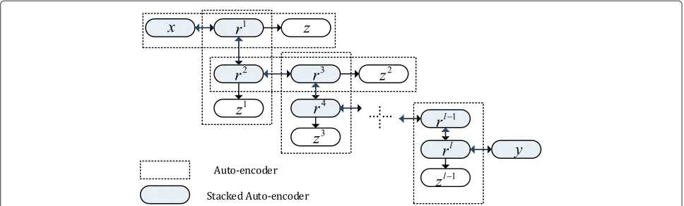
The auto-encoder [34] is the major component of SAE, as shown in Fig. 1, which is an unsupervised neural net-work that tries to force its output to equal its input. The architecture of the auto-encoder includes an input layer, a hidden layer, and an output layer. Suppose we have an input vectorx, we can get the coder by the parameters weightW1and biasb1,

r=fW1x+b1, (1)

and decode it by parametersW2,b2,

z=fW2r+b2, (2)

Fig. 1Stacked auto-encode and auto-encoder. Theblue partconstitutes a SAE, and everydashed boxis an auto-encoder

The loss function or energy function J(θ)measures the reconstructionzwhen given inputx,

J(θ)= 1 2M

M

m=1

z(m)−x(m)2

2, (3)

whereMis the number of training samples. The objec-tive is finding the parameters θ = W1,b1,W2,b2 which can minimize the difference between the

out-put and the inout-put over the whole training set X =

x(1),x(2),. . .,x(m),. . .,x(M), and this can be efficiently implemented via the stochastic gradient descent algo-rithm.

2.2 Stacked auto-encoders

A SAE [35] consists of multiple auto-encoders in which the code of each auto-encoder is the input of the succes-sive auto-encoder. A SAE contains one input layer at the bottom, more than one hidden layer in the middle, and one output layer at the top. We can get a representation or feature of the input data from every layer; the higher the layer is, the more abstract the feature is.

Suppose a training samplexand the corresponding label y. There are two steps to train a SAE, pre-training and fine-tuning [27]. The pre-training step is an unsupervised learning process which encodes the input in a hierarchical way, and fine-tuning is a supervised process which uses the label to optimize the whole network.

In the pre-training step, train an auto-encoder for the training sample x and get the code r(1), and then train the next auto-encoder for the coder(1), get the coder(2), use the code from the subjacent auto-encoder as the input of the next auto-encoder, and repeat until all subsequent hidden layersr(l) are obtained, forl = 1,· · ·,L,Lis the number of hidden layers in SAE.

After finishing the pre-training step, we use fine-tuning to optimize the whole network. Fine-tuning treats all lay-ers of SAE as a single neural network model; in each

iteration, it improves all the parameters from the last itera-tion, and it can improve the result of layer-wise training by a supervised strategy. Fine-tuning is performed by adding a final layer that represents the desired output. For classi-fication, the output is the label of the input sample. Then, the back propagation (BP) algorithm can be used to adjust or fine-tune the network weights in the same way as the feed-forward neural network.

Suppose we have a set of training samples

X = x(1),x(2),. . .,x(m),. . .,x(M), and the correspond-ing labels are y = y(1),y(2),. . .,y(m),. . .,y(M), where x(m) =

x₁(m),x(₂m),. . .,x_N(m) T, y(m) ∈ {1,· · ·,K}, for m= 1, 2,. . .,M,Mis the number of training samples,N is the unit number of the input layer, andKis the number of classes. The objective is to minimize the difference between the desired output and the real output, so the loss function for samplex(m)is defined as:

J

W,b;x(m),y(m) = 1 2

y(m)−z(m)2

2, (4)

The energy functionJ(W,b)over the whole training set is defined as:

J(W,b)= 1 M

M

m=1

JW,b;x(m),y(m) . (5) We minimize energy functionJ(W,b) to decrease the difference between the outputzand the true labelyover all the training samples. All the parameters are initial-ized randomly and updated by stochastic gradient descent (SGD), and each iteration of gradient descent updates the parametersW(l),b(l)in layerlas follows:

W(l):=W(l)−α ∂

∂W(l)J(W,b) (6) b(l):=b(l)−α ∂

propagation (BP) algorithm. The process of training SAE using gradient descent with the BP algorithm executes the coding procedure illustrated in Algorithm 1.

Algorithm 1Training SAE using SGD with BP algorithm coding procedure

Input:

Training setX=x(1),x(2),. . .,x(m),. . .,x(M); The corresponding labels y ∈ y(1),y(2),. . .,y(m),

. . .,y(M); Output:

ParametersW,bof SAE;

1: Forl=1, 2,· · ·,L,Lis the number of hidden layers 2: Computing all the hidden layers r(l,m) over the

whole training set using Eqs. (1), (2), and (3); 3: End For

4: Compute the output layerz(m);

5: Compute energy function J(W,b) over the whole training set:

J(W,b)= 1 M

M

m=1

JW,b;x(m),y(m) ;

6: Set ∂

∂W(l)J(W,b)=0,

∂

∂b(l)J(W,b)=0 7: Form=1,· · ·,M

8: Fori=1, 2,· · ·,nL+1,nL+1is the unit number in the output layer

9: δ(_iL+1)= −(∇J)f

z(_im) ; 10: End For

11: Forl=L,L−1,· · ·, 1

12: Fori = 1, 2,· · ·,nl,nl is the unit number in layerl

13: δ(_il)=

(W(l))Tδ(l+1) f

r(_il,m) ; 14: End For

15: End For

16: Compute the desired partial derivatives:

• ∂

∂b(l)J(W,b)=δ

(l+1)

• ∂

∂W(l)J(W,b)=δ

(l+1)_r(l,m)T ;

17: End For

18: Update the parameters: • W(l):=W(l)−α ∂

∂W(l)J(W,b) • b(l):=b(l)−α ∂

∂b(l)J(W,b);

19: Repeat line 4 to 18 untilW,bmeet the requirement;

SAE is a hybrid learning method, which includes both supervised and unsupervised steps. From optimization viewpoint, the unsupervised step, i.e., pre-training, can provide a relatively accurate initialization compared with random initialization, and from regularization viewpoint,

it can provide a prior about the training data (Y Ben-gio, I Goodfellow, A Courville: Deep Learning (2015), unpublished).

Each hidden layer in SAE is a representation of the input data. If the number of hidden units is larger than the dimensionality of input, the hidden layer projects the input data to a space with higher dimensionality, which will be able to discover correlations. Otherwise, the hidden layer is a compressed representation, which reduces dimensionality and eliminates redundancy. Cur-rently, there is no theory about how to define the numbers of hidden layers and the numbers of hidden units, and since the BP algorithm can be extended to apply to an arbi-trary number of layers, we can build a SAE with arbiarbi-trary depth by the BP algorithm.

There are many constraints that can be imposed into the deep network; a sparse SAE is imposing a sparsity con-straint on the hidden units, and then the auto-encoder will discover sparse features of the input data, just like the result of sparse representation.

3 Proposed method

Imaging spectrometers onboard satellites collect hyper-spectral images with hundreds of hyper-spectral bands in a narrow bandwidth with fixed sample intervals. However, not all channels are essentially useful for a specific appli-cation. Hence, in order to get a better classification map, it is necessary to extract an informative representation of the original spectral signature. We proposed a novel deep network, called contextual deep learning (CDL), which can extract effective spectral-spatial features from HSI directly and is especially effective for HSI classification.

The framework of this contextual deep structure con-tains one input layer, three kinds of hidden layers, and one output layer. The first hidden layer merges spectral infor-mation from adjacent pixels to add spatial inforinfor-mation in the processing pixels, the next (one or more) hidden layers learn the spectral feature elaborately, and the last hid-den layer is another spatial information which integrates a layer to smooth the information from the neighborhood. Suppose that a pixel or samplexin hyperspectral image isx = (x1,x2,. . .,xn0)T,n0is the number of the spectral

bands, andr(l)=

r₁(l),r₂(l),. . .,r(nll)

T

is the output of hid-den layer l or a representation from hidden layerl, and n_l is the number of the units in layerl. We will detail all pivotal layers in the following subsections.

3.1 Spatial information extraction

arep2pixels in U(x), then the output in the first hidden layer is given as:

r(1)=f

W(1)U(x)+b(1) , (8) where f(·) is the activation function, here is f(·) = 1, and the weightW(1)is used to decide how much spatial information to add. We carry on this operation for all the samples to get the first hidden layer of the contextual deep network, with the sample neighborhood as input. This layer is a new representation of the input HSI with spatial information in every pixel.

The weightW(1)is initialized via a 2-D Gauss filter, and because the input data have been normalized, we force the bias b(1) = 0. The only parameter in W(1) is the vari-ance of the 2-D Gauss filter, and we decide this parameter according to the spatial resolution of HSI.

3.2 Spectral feature mining

After finishing spatial information integration, we add more hidden layers to explore spectral features. The effects of spectral feature layers are reducing the redundancy spectral information, explore the correla-tion behind the input spectrum, and make the features more representative. We have already obtained r(1) =

r₁(1),r₂(1),. . .,r(n11) T

from the first hidden layer; suppose there aren2units in the second hidden layer,nl units in

thelth hidden layer. The outputr(l)=r₁(l),r(₂l),. . .,r(nll)

T

of layerlcan be computed by the following equation:

r(l)=f

W(l)r(l−1)+b(l) , (9) wherel = 2, 3,· · ·,L−1,W(l) is the weight matrix for projecting the units from layerl−1 to layerl, andb(l)is the bias. Here, we choose sigmoid function as the activation function of the layers for spectral feature mining.

Suppose we have a set of training samples

X = x(1),x(2),. . .,x(m),. . .,x(M), then the

corresponding output in layer l is R(l) =

r(l,1),r(l,2),. . .,r(l,m),. . .,h(l,M)

and the

correspond-ing labels are y = y(1)_,y(2)_{,. . .,y}(m)_{,. . .,y}(M)_{, where} x(m) = x(₁m),x(₂m),. . .,x(n0m)

T

, y(m) ∈ {1,· · ·,K}, for m= 1, 2,. . .,M,Nis the unit number of the input layer, andKis the number of classes.

In order to initializeW(l), we reconstructr(l−1,m)using r(l,m) as in Eq. (2) and minimize the average sum-of-squares error between r(l−1,m) and its reconstruction z(l−1,m)function :

JW(l),b(l) = 1 2M

M

m=1

r(l−1,m)−z(l−1,m)2 2. (10)

In order to get better representation, we impose a sparse constraint on the output of spectral hidden layers; in other words, we want most of the hidden units to be 0. The average activation of hidden unitiis defined as:

ˆ

ρi= 1 M

M

m=1

r(_il,m). (11) We would like to enforce the average activation equal to a sparsity parameterρ, which is close to zero. To achieve this, Kullback-Leibler (KL) divergence is used to penalize

ˆ

ρideviating fromρ:

KL(ρ|| ˆρi)=ρlog_ρρ_ˆ i +(

1−ρ)log1−ρ 1− ˆρi

. (12)

The overall cost function with a sparse term is:

J

W(l),b(l) =J

W(l),b(l) +β nl

i=1

KL(ρ|| ˆρj), (13)

whereβis the parameter to control sparsity. The objective is finding the parametersW(l),b(l) which can minimize the cost function over the whole training set, and this can be efficiently implemented via the stochastic gradient descent algorithm.

3.3 Feature smoothness

When we finish the spectral feature mining layers, we can use all units in layerL−1 as the spatial-spectral features.

(a) (b) (c) (d) (e)

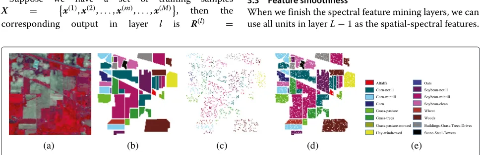
Table 1Classification accuracy ( %) for the Indian Pines image using 10 % training samples as shown in Fig. 3

Class Train Test SAE-LR LORSAL-MLL SOMP MPM-LBP CDL-MLR

1 5 49 93.33 100.0 100.0 100.0 100.0

2 143 1291 84.66 87.46 95.05 99.70 99.21

3 83 751 84.39 81.23 96.24 100.0 98.89

4 23 211 73.08 88.41 97.93 100.0 100.0

5 50 447 93.47 97.49 98.68 100.0 99.78

6 75 672 93.41 97.34 98.36 99.73 99.73

7 3 23 100.0 100.0 100.0 100.0 100.0

8 49 440 95.11 97.98 100.0 100.0 100.0

9 2 18 100.0 100.0 100.0 100.0 100.0

10 97 871 85.78 83.64 95.44 98.48 99.89

11 247 2221 83.46 86.31 91.80 98.74 99.22

12 61 553 81.62 91.79 91.71 99.35 98.99

13 21 191 98.52 100.0 100.0 100.0 100.0

14 129 1165 91.77 97.04 98.00 99.92 99.69

15 38 342 81.79 86.18 97.07 98.93 99.43

16 10 85 98.88 100.0 100.0 100.0 100.0

OA 86.85 87.18 92.60 97.50 98.23

AA 89.95 90.83 94.14 98.28 98.70

κ 0.8495 0.8536 0.9155 0.9715 0.9799

However, in order to smoothen the feature and suppress outliers in the spatial domain, we develop another layer. This layer uses the neighborhood of the unit from layer L−1 as the input and computes the output by:

r(L)=fW(L)Ur(L−1) +b(L) . (14) As in Eq. (8), the parameterW(L) is initialized via a 2-D Gauss filter, and we decide this parameter according to the spatial resolution of HSI.

3.4 Output layer

After finishing all the hidden layers, we add an output layer on the top of the deep network. In order to supervise the learning of spectral-spatial features, our output layer

is a multinomial logistic regression (MLR), also known as softmax regression, which is an extended version of logis-tic regression to solve multi-class classification problems. The output labelzfor samplexis given by:

z=g

1 K

k=1e(W

(L+1)₎T_r(L)

. (15)

The function g(·)returns to the position of the max com-ponent of input vector. Like all classifiers, the weight W(L−1) can be decided by minimizing a cost func-tion which minimizes the average sum-of-squares error between the resultszand the corresponding labelsyover all training samples.

3.5 Fine-tuning

After building all layers in a greedy layer-wise way, we use the fine-tuning approach in SAE to adjust all the parameters in our contextual deep learning by minimizing the following energy function using the coding procedure illustrated in Algorithm 1:

J_CDL(W,b)=min 1 M

M

k=1 1 2

z(m)−y(m)2+λ 2

L

l=1 W(l)2

F,

(16)

where J_CDL(W,b)is an energy function,Mis the number of training samples, the first term is an average sum-of-squares error term within all the samples, and the second term is the Frobenius norm that prevents over-fitting.

4 Experiments and performance comparisons

In this section, we evaluate the proposed method and other contrastive methods on several hyperspectral data sets which are all available online1. We use MATLAB 2014a on a computer with Intel Core i7 4.0 GHz CPU and 32 GB memory. For better comparison, please refer to the electronic versions of all the figures in these experiments.

(a) (b) (c) (d) (e)

(a) (b)

Fig. 4 aThe curve of OA obtained by different training sample percentages for the Indian Pines data set.bDistribution of the OA obtained by 30 different random realizations for the Indian Pines data set with 10 % training samples

4.1 Parameter setting

In the following experiments, the proposed contextual deep learning (CDL) algorithm with multinomial logis-tic regression (MLR) as output layer is compared to other widely used spectral-spatial classification methods, including stacked auto-encode with logistic regression (SAE-LR) [31], simultaneous orthogonal matching pursuit (SOMP) [18], augmented Lagrangian-multilevel logistic (LORSAL-MLL) [25], and maximizer of the posterior marginal by loopy belief propagation (MPM-LBP) [19]. SAE-LR processes HSI with principal component analy-sis (PCA) and uses blocks from PCA processed HSI as spatial features, then strings with spectral features as the input of SAE with LR as output layer. LORSAL-MLL uses logistic regression via splitting and augmented Lagrangian algorithm and encodes the spatial information by a mul-tilevel logistic prior. SOMP utilizes spatial information by a simultaneous versions of OMP. MPM-LBP uses LBP to include spatial information. All comparing methods are respectively implemented using the parameters given in relevant references aforementioned.

Furthermore, the following quality metrics are used to evaluate the performance of all methods. Overall accuracy (OA) refers to the percentage which is correctly classi-fied over all test samples, average accuracy (AA) shows the average value of classification accuracy for all classes, and Kappa coefficient (κ) is a statistical measurement of producer’s accuracy or user’s accuracy for classification result.

4.2 AVIRIS data set: Indian pines

This is a challenging scene with low spatial resolution, as shown in Fig. 2a. This data was gathered by AVIRIS sen-sor over north-western Indiana and consists of 145×145 pixels. After removing bands of water absorption, there are 200 spectral bands that cover from the visible light to SWIR with 20 m spatial resolution. There are 16 classes in the available ground truth, including two-thirds agricul-ture and one-third forest or other perennial vegetation.

First of all, we evaluate the classification accuracy of the proposed approach. We randomly selected 10 % per class for training and the remaining 90 % for testing in

(a) (b) (c) (d) (e)

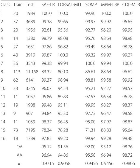
Table 2Classification accuracy ( %) for the Salinas image using 1 % training samples as shown in Fig. 6

Class Train Test SAE-LR LORSAL-MLL SOMP MPM-LBP CDL-MLR

1 20 1989 100.0 100.0 99.90 100.0 100.0

2 37 3689 99.38 99.65 99.97 99.92 96.65

3 20 1956 92.61 95.56 92.77 96.20 99.95

4 14 1380 98.79 98.08 95.76 98.64 98.98

5 27 1651 97.86 96.82 99.49 98.64 98.78

6 40 3919 99.87 100.0 99.32 99.97 99.27

7 36 3543 99.38 99.94 100.0 99.94 100.0

8 113 11,158 83.32 80.10 86.61 88.64 96.62

9 62 6141 99.37 98.94 98.81 99.58 99.92

10 33 3245 96.07 94.54 95.21 92.27 98.57

11 11 1057 95.86 89.83 97.53 96.54 96.78

12 19 1908 99.48 95.11 99.95 98.27 98.37

13 9 907 94.84 95.30 97.73 96.47 98.58

14 11 1059 98.37 96.45 95.00 97.97 98.87

15 73 7195 78.34 78.28 71.31 88.83 95.64

16 18 1789 97.85 99.20 99.94 99.28 99.48

OA 95.12 91.56 92.00 95.12 98.26

AA 96.94 94.86 95.58 96.94 98.72

κ 0.9715 0.9058 0.9456 0.9456 0.9806

all those methods; the numbers of the training and test sets are shown in Table 1. SAE-LR uses the first six prin-cipal components to get spatial features, and the window size is 7×7; in the SAE, we have used 180 units in the first hidden layer and 100 units in the second hidden layer. SOMP uses a 9×9 square window, and LORSAL-MLL and MPM-LBP use the parameters for this data in the origi-nal papers. For CDL-MLR, we use four hidden layers; the first one is a spatial information layer with a window size of 7×7, with 50 units in next hidden layer, 80 units in the third hidden layer, and 7×7 square window in the last hid-den layer. According to the previous studies, the number of hidden nodes is more important than the number of hidden layers. Considering computational complexity, we

operated tons of experiments under various unit numbers within 100 and chose a set which can give steady perfor-mance. Classification results of AVIRIS Indian Pines data using different algorithms are shown in Fig. 3; sub-figures from left to right are results from SAE-LR, LORSAL-MLL, SOMP, MPM-LBP, and CDL-MLR, respectively. The accu-racy of all classification methods for each class along with the overall accuracy and the kappa coefficient is given in Table 1.

Due to the low spatial resolution of this data set, the presence of mixed pixels are the leading challenge for clas-sification. Results confirm that the spectral-spatial classi-fication using learning-based feature extraction is able to improve the classification accuracy considerably; that is because spatial features can help to significantly prevent salt-and-pepper noise in the result of pixel-wise classifica-tion. However, how much spatial information to use is a tricky problem, and too much spatial information would suppress small structures and cause terrible classification results. For this data set, considering the low spatial reso-lution, we use a smaller spatial window. Table 1 shows the accuracy of different methods wherein the first column is the class label. From the table, for this challenging classi-fication scenario, the best result is from CDL-MLR with OA=98.23 %, AA=98.70 %, andκ=0.9799.

Next, we perform experiments to examine the effect of the number of training samples. All the parameters are fixed except the numbers of training samples per class. The classification OA is plotted under various percentages of samples in Fig. 4a, where the x-axis denotes the per-centage of training samples per class and they-axis is OA averaged over five times. From the figure, we can tell that OA monotonically increases with the size of the training set for every algorithm. The CDL method always outper-forms other methods and even more significantly when there is a small training set. When the number of train-ing samples is more than 20 % of each class in the ground truth, the OA is tending towards stability.

Finally, we compare the stability of all classification methods. We randomly choose 10 % of the labeled sam-ples as the training set and randomly execute 30 tests

(a) (b) (c) (d) (e)

(a) (b)

Fig. 7 aThe curve of OA obtained by different window sizes for the Salinas data set.bThe curve of OA obtained by different layers for the Salinas data set with different training sample percentages

for all algorithms. The functions of probability density of OA are presented in Fig. 4b. From the figure, the average classification rate is the highest for CDL-MLR, which is consistent with the results in Fig. 3. Furthermore, the low-est variance is from CDL-MLR, underlining its improved robustness against a particular choice of training samples.

4.3 AVIRIS data set: Salinas

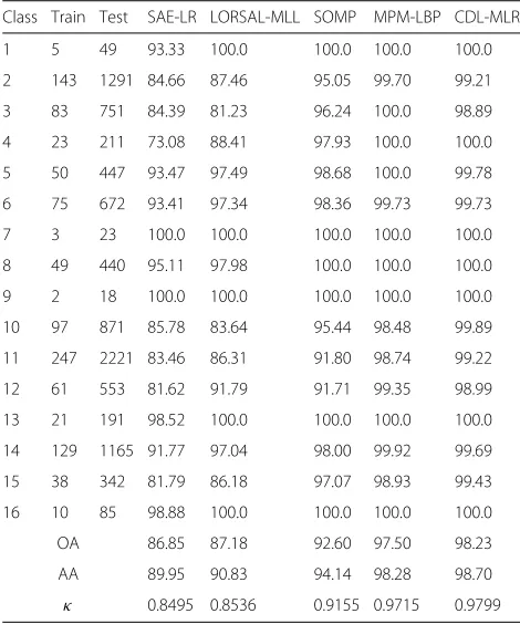
As shown in Fig. 5, this data was acquired by the AVIRIS sensor over Salinas Valley, California, and consists of 512×217 pixels. There are 224 spectral bands covering from the visible light to SWIR with 3.7 m spatial resolu-tion. After discarding water absorption bands, 204 bands were left. Salinas ground truth contains 16 classes and includes vegetables, bare soils, and vineyard fields.

We randomly selected only 1 % per class for training and the remaining 99 % for testing in all those methods; the numbers of the training and test sets are shown in Table 2. SAE-LR uses the first six principal components to get spatial features, and the window size is 7×7. In the SAE, we have used 200 units in the first hidden layer

and 120 units in the second hidden layer. SOMP uses a

9×9 square window, and LORSAL-MLL and MPM-LBP

use the parameters for this data in the original papers. For CDL-MLR, we use four hidden layers; the first one is a spatial information layer with a window size of 7×7, with 150 units in next hidden layer, 100 units in the third hidden layer, and a 7×7 square window in the last hid-den layer. Classification results of Salinas data are shown in Fig. 6. Sub-figures from left to right are results from SAE-LR, LORSAL-MLL, SOMP, MPM-LBP, and CDL-MLR, respectively. The accuracy of all classifications for each class along with the overall accuracy and the kappa coefficient is given in Table 2. From the table, for this challenging classification scenario, the best result is from

CDL-MLR with OA = 98.26 %, AA = 98.72 %, and

κ=0.9806.

Next, we perform experiments to examine the effect of the window size of the spatial layer. All the parameters are fixed except the window size. The classification OA is plotted under various percentages of samples in Fig. 7a, where thex-axis denotes the window size and they-axis

(a) (b) (c) (d) (e)

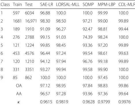
Table 3Classification accuracy ( %) for the University of Pavia image using 9 % training samples as shown in Fig. 9

Class Train Test SAE-LR LORSAL-MLL SOMP MPM-LBP CDL-MLR

1 597 6034 96.88 100.0 100.0 99.99 100.0

2 1681 16,971 98.30 98.50 97.21 99.00 99.89

3 189 1910 91.09 96.27 92.47 98.81 99.44

4 276 2788 99.15 91.03 74.39 98.24 100.0

5 121 1224 99.85 98.45 93.36 97.20 99.89

6 453 4576 96.44 97.24 99.54 98.61 99.63

7 120 1210 94.12 97.94 96.76 99.18 99.89

8 331 3351 93.27 99.94 99.58 99.90 100.0

9 85 862 100.0 100.0 100.0 97.45 100.0

OA 97.12 98.95 97.84 98.83 99.86

AA 96.57 97.28 93.96 97.36 99.64

κ 0.9615 0.9819 0.9628 0.9799 0.9976

is the averaged OA over five times. From the figure, we can tell that every curve of OA monotonically increases with the window size, but when the window size is too big, the OA does not increase anymore; that is because the deep network gives the outside pixels in the window zero weights.

At last, we investigate the effect of every layer and show the results in Fig. 7b. First, we use only one hidden layer for extracting spectral features, then two hidden layers, then two hidden layers with a spatial feature layer, and last, all four layers. We use 0-1-1-0 to express that we use the second and the third layers. The classification OA is plot-ted under various percentages of samples in Fig. 7b, where thex-axis denotes the percentage of training samples per class and they-axis is averaged OA over five times. From the figure, we can see the contribution of each layer, and the first hidden layer (blue line) for spatial feature mining is very effective and enhances the average OA in a big step.

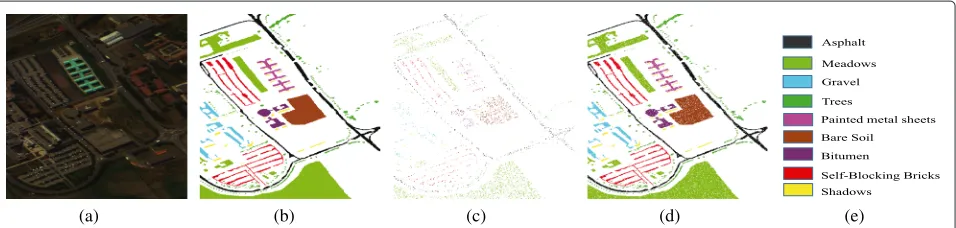
4.4 ROSIS urban data: University of Pavia

As shown in Fig. 8, this data set was collected by the ROSIS sensor over Pavia, northern Italy, and consists

610×340 pixels. There are 103 spectral bands with 1.3 m spatial resolution. The available ground truth contains nine classes and includes vegetables, soils, and buildings.

For this data, we randomly pick 9 % labeled samples in each class as training samples and the remainder as test samples. Numbers of training and test sets can be seen in Table 3. SAE-LR uses the first four principal components as bands for spatial feature extraction, and the window size is 9×9. In the SAE, we have used 180 units in the first hidden layer and 100 units in the second hidden layer. SOMP, LORSAL-MLL, and MPM-LBP use the parame-ters for this data in the original papers. For CDL-MLR, we use four hidden layers, the first one with a window size of 19×19, with 50 units in the next hidden layer, 80 units in the last hidden layer, and a 19×19 square window in the last hidden layer. The classification results using different algorithms are shown in Fig. 9. The accuracy of all classifications for each class along with the over-all accuracy and the kappa coefficient is given in Table 3. The best result from the table is from CDL-MLR with OA=99.86 %.

4.5 Discussion

Overall, the experiments suggest that incorporation of spatial information improves the classification perfor-mance, and the proposed CDL-MLR is competitive with some of the best available spectral-spatial methods for hyperspectral image classification.

In our algorithm, the most important part is the fea-ture representation which affects the performance of HSI classification. We use a deep learning algorithm to learn the spectral and spatial features, and the number of hid-den units is an important parameter. Currently, there is no theory analysis about how to decide on this parameter. Such analysis is beyond the scope of this work and better left for consideration of specific applications.

5 Conclusions

In this paper, we introduced a novel feature mining algo-rithm, contextual deep learning, which is especially effec-tive for HSI classification. Learning both the spatial and

(a) (b) (c) (d) (e)

spectral features through contextual deep learning, the accuracy of the classifier can be improved dramatically.

Compared with other classification methods, the major advantage of the proposed method is that it is able to obtain high-quality spectral and spatial features, using just a few training samples and a simple classifier, and outstanding classification results can be achieved. Thus, the proposed method will be quite useful in real applica-tions due to its superior accuracy. Since tons of unlabeled data are available in HSI classification, a topic of future research is to investigate how to use unlabeled samples in this deep network and develop a semisupervised feature learning method for HSI classification.

Endnote

1_{Available online: http://www.ehu.es/ccwintco/index.} php?title=Hyperspectral_Remote_Sensing_Scenes.

Competing interests

The authors declare that they have no competing interests.

Acknowledgements

The authors would like to thank Purdue University, the University of Pavia, and the HySenS project for kindly providing the hyperspectral images in this paper. The authors would also like to thank the anonymous reviewers for helpful comments and constructive suggestions.

Received: 17 December 2014 Accepted: 11 May 2015

References

1. C-I Chang,Hyperspectral Data Exploitation: Theory and Applications. (John Wiley & Sons, Hoboken, New Jersey, 2007)

2. DA Landgrebe,Signal Theory Methods in Multispectral Remote Sensing, vol. 29. (John Wiley & Sons, Hoboken, New Jersey, 2005)

3. F Melgani, L Bruzzone, Classification of hyperspectral remote sensing images with support vector machines. IEEE Trans. Geosci. Remote Sens. 42(8), 1778–1790 (2004). [doi:10.1109/TGRS.2004.831865]

4. Y Tarabalka, M Fauvel, J Chanussot, JA Benediktsson, SVM-and MRF-based method for accurate classification of hyperspectral images. IEEE Geosci. Remote Sens. Lett.7(4), 736–740 (2010)

5. G Hughes, On the mean accuracy of statistical pattern recognizers. IEEE Trans. Inform. Theory.14(1), 55–63 (1968). [doi:10.1109/TIT.1968.1054102] 6. G Camps-Valls, L Bruzzone, Kernel-based methods for hyperspectral

image classification. IEEE Trans. Geosci. Remote Sens.43(6), 1351–1362 (2005). [doi:10.1109/TGRS.2005.846154]

7. Y Gu, C Wang, D You, Y Zhang, S Wang, Y Zhang, Representative multiple kernel learning for classification in hyperspectral imagery. IEEE Trans. Geosci. Remote Sens.50(7), 2852–2865 (2012).

[doi:10.1109/TGRS.2005.846154]

8. J Li, PR Marpu, A Plaza, JM Bioucas-Dias, JA Benediktsson, Generalized composite kernel framework for hyperspectral image classification. IEEE Trans. Geosci. Remote Sens.51(9), 4816–4829 (2013).

[doi:10.1109/TGRS.2005.846154]

9. RM Willett, MF Duarte, MA Davenport, RG Baraniuk, Sparsity and structure in hyperspectral imaging: sensing, reconstruction, and target detection. IEEE Signal Process. Mag.31(1), 116–126 (2014).

[doi:10.1109/MSP.2013.2279507]

10. P Ghamisi, JA Benediktsson, JR Sveinsson, Automatic spectral-spatial classification framework based on attribute profiles and supervised feature extraction. IEEE Trans. Geosci. Remote Sens.52(9), 5771–5782. [doi:10.1109/TGRS.2013.2292544]

11. P Ghamisi, JA Benediktsson, G Cavallaro, A Plaza, Automatic framework for spectral-spatial classification based on supervised feature extraction and morphological attribute profiles. IEEE J. Sel. Topics Appl. Earth Observ. Remote Sens.7(6), 2147–2160 (2014). [doi:10.1109/JSTARS.2014.2298876]

12. J Li, H Zhang, L Zhang, Supervised segmentation of very high resolution images by the use of extended morphological attribute profiles and a sparse transform. IEEE Geosci. Remote Sens. Lett.11(8), 1409–1413 (2014) 13. B Song, J Li, M Dalla Mura, P Li, A Plaza, JM Bioucas-Dias, J Atli

Benediktsson, J Chanussot, Remotely sensed image classification using sparse representations of morphological attribute profiles. IEEE Trans. Geosci. Remote Sens.52(8), 5122–5136 (2014)

14. P Ghamisi, M Dalla Mura, JA Benediktsson, A survey on spectral-spatial classification techniques based on attribute profiles. IEEE Trans. Geosci. Remote Sens.53(5), 2335–2353 (2015)

15. Q Zhang, Y Tian, Y Yang, C Pan, Automatic spatial-spectral feature selection for hyperspectral image via discriminative sparse multimodal learning. IEEE Trans. Geosci. Remote Sens.53(1), 261–279 (2015). [doi:10.1109/TGRS.2014.2321405]

16. Y Zhou, J Peng, C Chen, Extreme learning machine with composite kernels for hyperspectral image classification. IEEE J. Sel. Topics Appl. Earth Observ. Remote Sens.PP(99), 1–10 (2014)

17. Y Zhang, S Prasad, Locality preserving composite kernel feature extraction for multi-source geospatial image analysis. IEEE J. Sel. Topics Appl. Earth Observ. Remote Sens.PP(99), 1–8 (2014)

18. Y Chen, NM Nasrabadi, TD Tran, Hyperspectral image classification via kernel sparse representation. IEEE Trans. Geosci. Remote Sens.51(1), 217–231 (2013). [doi:10.1109/TGRS.2012.2201730]

19. J Li, JM Bioucas-Dias, A Plaza, Spectral-spatial classification of hyperspectral data using loopy belief propagation and active learning. IEEE Trans. Geosci. Remote Sens.51(2), 844–856 (2013).

[doi:10.1109/TGRS.2012.2205263]

20. G Camps-Valls, D Tuia, L Bruzzone, J Atli Benediktsson, Advances in hyperspectral image classification: Earth monitoring with statistical learning methods. IEEE Signal Process. Mag.31(1), 45–54 (2014). [doi:10.1109/MSP.2013.2279179]

21. L Cheng-Hsuan, K Bor-Chen, L Chin-Teng, H Chih-Sheng, A

spatial-contextual support vector machine for remotely sensed image classification. IEEE Trans. Geosci. Remote Sens.50(3), 784–799 (2012). [doi:10.1109/TGRS.2011.2162246]

22. G Moser, SB Serpico, Combining support vector machines and Markov random fields in an integrated framework for contextual image classification. IEEE Trans. Geosci. Remote Sens.51(5), 2734–2752 (2013). [doi:110.1109/TGRS.2012.2211882]

23. G Moser, SB Serpico, JA Benediktsson, Land-cover mapping by Markov modeling of spatial-contextual information in very-high-resolution remote sensing images. Proc. IEEE.101(3), 631–651 (2013). [doi:10.1109/JPROC.2012.2211551]

24. Y Tarabalka,Classification of hyperspectral data using spectral-spatial approaches. (Thesis, University of Iceland and Grenoble Institute of Technology, 2010)

25. J Li, JM Bioucas-Dias, A Plaza, Hyperspectral image segmentation using a new Bayesian approach with active learning. IEEE Trans. Geosci. Remote Sens.49(10), 3947–3960 (2011). [doi:10.1109/TGRS.2011.2128330] 26. Y Sun, X Wang, X Tang, inIEEE Conf. Comput. Vision and Pattern

Recognition. Deep learning face representation from predicting 10,000 classes (IEEE Columbus, OH, USA, 23–28 June 2014), pp. 1891–1898. [doi:10.1109/CVPR.2014.244]

27. D Yu, L Deng, GE Dahl, inNIPS 2010 Workshop on Deep Learning and Unsupervised Feature Learning. Roles of pre-training and fine-tuning in context-dependent DBN-HMMs for real-world speech recognition (Whistler, BC, Canada, 10 December 2010)

28. F Zhang, B Du, L Zhang, Saliency-guided unsupervised feature learning for scene classification. IEEE Trans. Geosci. Remote Sens.53(4), 2175–2184. IEEE

29. AM Cheriyadat, Unsupervised feature learning for aerial scene classification. IEEE Trans. Geosci. Remote Sens.52(1), 439–451. [doi:10.1109/TGRS.2013.2241444]

30. H Xie, S Wang, K Liu, S Lin, B Hou, inIEEE International Geoscience and Remote Sensing Symposium (IGARSS). Multilayer feature learning for polarimetric synthetic radar data classification (IEEE Quebec City, 2014), pp. 2818–2821

32. Z Lin, Y Chen, X Zhao, G Wang, inProc. 9th Int. Conf. Inf., Commun. Signal Process. (ICICS). Spectral-spatial classification of hyperspectral image using autoencoders, (Dec. 2013), pp. 1–5. [doi:10.1109/ICICS.2013.6782778] 33. GE Hinton, S Osindero, Y-W Teh, A fast learning algorithm for deep belief

nets. Neural Comput.18(7), 1527–1554 (2006). [doi:10.1162/neco.2006.18.7.1527]

34. GE Hinton, RS Zemel, inAdvances in Neural Information Processing Systems 6, ed. by JD Cowan, G Tesauro, and J Alspector. Autoencoders, minimum description length and helmholtz free energy (NIPS, 1993), pp. 3–10 35. P Vincent, H Larochelle, I Lajoie, Y Bengio, P-A Manzagol, Stacked

denoising autoencoders: learning useful representations in a deep network with a local denoising criterion. J. Mach. Learn. Res.11, 3371–3408 (2010)

Submit your manuscript to a

journal and benefi t from:

7 Convenient online submission

7 Rigorous peer review

7 Immediate publication on acceptance

7 Open access: articles freely available online 7 High visibility within the fi eld

7 Retaining the copyright to your article