Automatic Identification of Algae using Low-cost Multispectral Fluorescence Digital Microscopy, Hierarchical Classification & Deep Learning

(1)

Automatic Identification of Algae

using Low-cost Multispectral

Fluorescence Digital Microscopy,

Hierarchical Classification

& Deep Learning

by

Jason Deglint

A thesis

presented to the University of Waterloo in fulfillment of the

thesis requirement for the degree of Doctor of Philosophy

in

Systems Design Engineering

Waterloo, Ontario, Canada, 2019

(2)

Examining Committee Membership

The following served on the Examining Committee for this thesis. The decision of the Examining Committee is by majority vote.

External Examiner: Stefan C. Kremer Professor

School of Computer Science, University of Guelph

Supervisor: Alexander Wong

Associate Professor

Systems Design Engineering, University of Waterloo

Internal Member: Katharine Scott Assistant Professor

Internal Member: John Zelek

Associate Professor

Internal-External Member: Zhou Wang Professor

(3)

Author’s Declaration

This thesis consists of material all of which I authored or co-authored: see Statement of Contributions included in the thesis. This is a true copy of the thesis, including any required final revisions, as accepted by my examiners.

(4)

Statement of Contributions

There are three journal papers that make up parts of this thesis. Each paper will outline the contributions of each author that are relevant to the work presented in this thesis. I am the primary author and major contributor of all these papers.

The first journal paper was published in the Journal of Computational Vision and Imaging Systems in 2018 and was titled SAMSON: Spectral Absorption-fluorescence Mi-croscopy System for ON-site-imaging of algae. The authors on this paper were Jason L. Deglint (JLD), Lyndon Tang (LT), Yitian Wang (YW), Chao Jin (CJ) and Alexander Wong (AW). This paper published the implementation of the imaging system designed by JLD, CJ and AW, as discussed in Section4.4. The printed circuit board (PCB) and the 3D printed frame from this paper are presented in Section 4.4.2 of this thesis. The PCB and 3D print was designed by JLD and LT while LT implemented these designs. The graphical user interface (GUI) in this paper is presented in Section4.4.3 of this thesis. The GUI was designed by JLD and YW while YW implemented the design.

The second journal paper was published in IEEE Access in 2018 and was titledThe Fea-sibility of Automated Identification of Six Algae Types using Feed-forward Neural Networks and Fluorescence-based Spectral-morphological Features. The authors on this paper were JLD, Angela Chao (AC), CJ, and AW. This paper demonstrated that features could be extracted from multispectral fluorescence data and used as input into a feedforward neural network for classification of six algae. JLD and AC implemented the imaging apparatus in this paper, which inspired the work presented in Section4.4.2. The feedforward model in this paper inspired the work in Section5.2.1, and the data preprocessing in this paper was similar to Section 6.3. All the data collection and analysis in this paper are independent of this thesis.

The third paper was published in Springer: Lecture Notes in Computer Science in 2019 and was titledInvestigating the Automatic Classification of Algae via Deep Residual Learn-ing. The authors of this paper were JLD, CJ, and AW. The residual network developed for this paper is the same model presented in Section 5.2.2 and was designed by JLD and AW. All the data collection and analysis in this paper are independent of this thesis.

(5)

Abstract

Harmful algae blooms (HABs) can produce lethal toxins and are a rising global con-cern. In response to this threat, many organizations are monitoring algae populations to determine if a water body might be contaminated. However, identifying algae types in a water sample requires a human expert, a taxonomist, to manually identify organisms using an optical microscope. This is a tedious, time-consuming process that is prone to human error and bias. Since many facilities lack on-site taxonomists, they must ship their water samples off site, further adding to the analysis time.

Given the urgency of this problem, this thesis hypothesizes that multispectral fluores-cence microscopy with a deep learning hierarchical classification structure is the optimal method to automatically identify algae in water on-site. To test this hypothesis, a low-cost system was designed and built which was able generate one brightfield image and four flu-orescence images. Each of the four fluflu-orescence images was designed to target a different pigment in algae, resulting in a unique autofluorescence spectral fingerprint for different phyla groups.

To complement this hardware system, a software framework was designed and devel-oped. This framework used the prior taxonomic structure of algae to create a hierarchical classification structure. This hierarchical classifier divided the classification task into three steps which were phylum, genus, and species level classification. Deep learning models were used at each branch of this hierarchical classifier allowing the optimal set of features to be implicitly learned from the input data.

In order to test the efficacy of the proposed hardware system and corresponding software framework, a dataset of nine algae from 4 different phyla groups was created. A number of preprocessing steps were required to prepare the data for analysis. These steps were flat field correction, thresholding and cropping. With this multispectral imaging data, a number of spatial and spectral features were extracted for use in the feature-extraction-based models.

This dataset was used to determine the relative performance of 12 different model architectures, and the proposed multispectral hierarchical deep learning approach achieved the top classification accuracy of 97% to the species level. Further inspection revealed that a traditional feature extraction method was able to achieve 95% to the phyla level when only using the multispectral fluorescence data. These observations strongly support that: (1) the proposed low-cost multispectral fluorescence imaging system, and (2) the proposed hierarchical structure based on the taxonomy prior, in combination with (3) deep learning methods for feature learning, is an effective method to automatically classify algae.

(6)

Acknowledgements

Completing a PhD is a substantial commitment and as with any journey, has many ups and down as well as twists and turns. There is no way I could have completed my dissertation without the guidance, love and support of many individuals and organizations whom I am honoured to acknowledge now. All the people mentioned below helped me get to where I am today.

First I want to thank Alexander Wong, my supervisor and research dad. Without Alex I wouldn’t have begun a PhD as he encouraged me to apply for NSERC and supported me in preparing my application which in turn allowed me to pursue a full-time PhD without financial burden. Thank you Alex for taking me on as your student and for allowing me the freedom to select my research topic and pursue my passion for entrepreneurship. I greatly value your honesty and guidance to help me think critically and objectively about my research.

Secondly I want to thank Chao Jin, my co-supervisor and friend. When I started my PhD in September 2016, I intended to pursue research in multispectral imaging of art paintings. After chatting extensively with Chao I decided to switch my PhD topic to focus on water. Thank you Chao for your support and conversations about developing imaging technology to ensure clean drinking water, as this has a direct impact on people’s lives.

Next I want to thank my dear wife, Taylor Jade. Thank you Taylor for your unwavering support in my studies and encouraging me in my entrepreneurial ambitions. I couldn’t have completed this PhD without you.

Thank you to de Gasp´e Beaubien Foundation for hosting AquaHacking and for gen-erously awarding our team (Alex, Chao and myself) the first place prize in 2017. This was the beginning of my entrepreneurial journey in the water industry and the origin of Blue Lion Labs. Winning AquaHacking accelerated my path as an entrepreneur and was a springboard that opened doors into Toronto, Montreal, Vancouver, China and the USA. Thank you Angela Chao, Lyndon Tang, and Yitian Wang (co-ops and URAs) who assisted with my research. I value the work you contributed to my thesis and am grateful for your time. Also, thank you Heather Roshon at the CPCC for all your hard work preparing samples and answering all my questions.

Thank you NSERC for awarding me a full scholarship and thank you University of Waterloo for hosting me as a student. Thank you Velocity for providing free workspace and mentorship for Blue Lion Labs. Thank you to my committee for your time and energy. Finally, thank you to all my family and friends who supported me in my PhD studies in one way or another. Specifically, I want thank my mom (Jane Deglint) for proofreading this thesis for spelling and grammar.

(7)

Dedication

ded · i ·cate: devote (time, effort, or oneself) to a particular task or purpose. I have been given a gift.

The gift of freedom

to explore my interests and to pursue my passions. The gift of opportunity

to study and research this universe. The gift of time

to ponder and travel.

With this gift comes responsibility. Responsibility to work

on meaningful solutions that build and create. Responsibility to share

my knowledge and discoveries. Responsibility to serve

those in need and my fellow man. This responsibility calls me to devote myself.

Devote myself to constant gradual improvement

based on ruthlessly seeking reality and taking ownership of my actions. Devote myself to build up others

by encouraging them and treating each person with respect and dignity. Devote myself to creating a better world

not out of payment for the gift, but out of thankfulness for it.

First off, I dedicate this work to my amazing wife Taylor Jade. You have encouraged me to pursue reality and held me accountable to a higher standard. I admire your love for life and internal joy that you share with others. You can do anything.

Secondly, I dedicate this work to the spirit of innovation and exploration that each person has. May it take us further than we can ever imagine. May it allow us to steward our home and care for each other.

(8)

List of Figures

1.1 The Moderate Resolution Imaging Spectroradiometer (MODIS) on the Aqua satellite showing a harmful algae bloom (HAB) on Lake Erie on October 9, 2011 [2]. . . 2

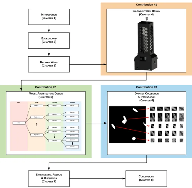
1.2 This thesis is composed of 8 main chapters. After this introductory Chapter 1, Chapter 2 goes into detail of the background of HABs and algae, while Chapter 3 present the current methods of automatic identification of algae. Chapter 4 presents the hardware contribution of this thesis and Chapter 5 describes the software framework. Then, in Chapter 6 a dataset is created in order to evaluate the efficacy of the Contribution 1 and Contribution 2. In Chapter 7 the results are presented and in Chapter 8 the final conclusions are discussed. . . 4

2.1 The standard method of identifying and enumerating microalgae consists of three main steps which are: (1) sample preparation, (2) classification, and (3) enumerating. The three main methods to condense the sample are filtration, using centrifugation and sedimentation [21]. . . 9

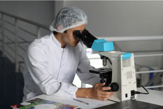
2.2 Manual identification of algae requires a human expert, a taxonomist, to manually look through a microscope and classify all the organisms present in a water sample. This method requires years of experience and is both time-consuming and tedious. . . 10

3.1 As observed in Table 3.1, different phyla of algae contain different antenna pigments [21]. Here the major pigments are shown on a single plot [32]. Note how different pigment are spread across different parts of the visible spectrum. . . 14

(14)

3.2 The absorption of light of a solution can be measured by passing a known broadband light source through the solution and measuring the transmitted signal with a spectrometer. . . 20

3.3 The absorption of algae for different phyla groups reported by Lee et al.

(top) [49] and Held et al. (bottom) [50]. . . 21

3.4 A fluorescence spectra can be measured by using a broadband light source which passes through a narrow bandpass filter to isolate the excitation wave-lengths. This excitation light enters the sample, causes the sample to flu-oresce, and emits a lower energy light signal. This lower energy light gets filtered by an additional highpass filter and then measured by a spectrometer. 22

3.5 The excitation spectra from 400 nm - 650 nm was reported by Poryvkina

et al. [51] (top) and Gsponer et al. [52] (bottom). These spectra reveal significant differences in the excitation wavelengths for different phyla of algae.. . . 23

3.6 The emission spectra ofPorphyridium sp. by Frenchet al. [53] (top) and the emission spectral of four common algae from three phyla groups by Millie

et al. [54]. These spectra show that different algae have different emission spectra which is the result of these algae having different different pigments. Notice the wavelength range in this figure compared to the wavelength range in Figure 3.5. Since the emission spectra is at a lower energy, the spectra will be at a higher wavelength. . . 25

3.7 The excitation and emission spectra ofMicrocystis sp. measured by Gsponer

et al. (top) [52] and by Heldet al. (bottom) [50]. While the emission spectra is very similar, the excitation spectra varies between these two authors. . . 26

4.1 The optimal LEDs (top) where chosen based from the excitation spectra presented by Poryvkinaet al [51] and Gsponeret al. [52] (second from top). Furthermore, the transmission of the high-pass filter (third from top) was selected based off the emission data presented by Frenchet al [53] and Millie

et al. [54] (bottom).. . . 38

4.2 A 2700 K LED (top) is used as a light source for the brightfield imaging modality. This LED will interact with the absorption spectra of different algae, a few of which are presented by Leeet al. [49] (middle). The highpass filter (bottom) then blocks any light lower than 635 nm. . . 40

(15)

4.3 The optical system of the proposed imaging device allows the camera sensor to capture a single brightfield image as well as four fluorescence images at different excitation wavelengths. It is this configuration that will be used to generate a dataset which can be fed into a software framework for automatic identification of algae. . . 41

4.4 Left: Using the USAF 1951 chart a spatial resolution of 0.65 um / pixel was able to be achieved. Right: This is sufficient to measure single-celled

microcystis aeruginosa which is known to be 3-7 um [65]. This microcystis aeruginosa from the dataset in Chapter 6 is 10 pixels in diameter, resulting in a diameter of 6.5 um. . . 43

4.5 The proposed imaging system was built using off the shelf components and housed by a 3D printed frame. The user places the water sample in the imaging path and then adjust the focus with the focusing knob. All control over the illumination sources and sensor of SAMSON is done through the graphical user interface (Fig. 4.6). . . 45

4.6 The graphical user interface (GUI) enables the flexible selection of different illumination sources and changes in exposure time of the sensor, during the process of viewing the water sample in real-time.. . . 46

5.1 The feedforward neural network architecture used in feature extraction based models. The extracted features are input into the model. The data propa-gates through the network in order to classify a given type of algae. . . 51

5.2 A two layer residual block as proposed by He et al. [79] where the convo-lutional layers are in green, the batch normalization layers are in blue, and the ReLU layers are in yellow. This basic building block is repeated in the proposed model as seen in Figure 5.3. . . 53

5.3 The proposed deep convolutional neural network architecture for algae clas-sification from multispectral imaging data. The architecture is based on a ResNet-18 architecture [79] with the input layer designed to take in a stack of multispectral images, and the output layer designed to predict the type of algae in the imaging stack. The feature extraction component of the architecture was pretrained using the ImageNet dataset [81, 82]. . . 54

(16)

5.4 The proposed hierarchical structure is broken into four levels: the base level, the phyla, level, the genera level, and the species level. Building a machine learning model in a hierarchical manner allows online learning and explainability, both of which are important in a regulated industry such as drinking water treatment plants.. . . 56

6.1 The taxonomic breakdown of the nine types of algae used to test the pro-posed hardware system and software framework. These nine algae come from four different phyla groups and were purchased from the Canadian Phyco-logical Culture Centre (CPCC). The physical appearance of these nine algae can be seen in Figure 6.2. . . 62

6.2 The nine types of algae used to test the proposed hardware system and soft-ware framework. Note that some algae types are very similar in appearance, as observed in the filamentous algae (top row) as well as the single celled algae (bottom row). . . 64

6.3 The raw images go through a three step process in order to create cropped images ready to be used by an image classifier. These steps are flat field correction, thresholding and cropping.. . . 65

6.4 Flat field correction takes the raw camera image and corrects for noise, illuminations and optical distortions [33]. . . 66

6.5 The highest contrast image of the flat field corrected images was manually chosen to be used in the thresholding task. Thresholding results in a binary mask which distinguishes the foreground and background from each other. 67

6.6 Given the binary mask which separates the foreground and the background, each foreground object can be cropped, resulting in a multispectral cropped image. . . 68

6.7 An example brightfield image crop for each of the nine algae types. Note how certain algae are significantly smaller in scale compared to other algae. 69

6.8 The brightfield cropped images were used to generate a set of spatial features using Fourier descriptors, Hu’s invariant moments, geometric shape features, and texture features. The four band fluorescence spectral image was used to generate spectral features. . . 70

6.9 A total of 6330 segmented and cropped multispectral images were generated from the raw image collected from the imaging system. The class distribu-tion of the nine types of algae can be seen above. . . 74

(17)

7.1 The nine algae types from four phyla groups at four excitation wavelengths (445 nm, 500 nm, 545 nm, and 620 nm) as well as the single brightfield image. This data was collected with the imaging device from Chapter 4 and preprocessed using the methods in Chapter 6. The average numerical values of the entire dataset can be seen in Figure 7.2. . . 77

7.2 The multispectral emission spectra from nine types of algae when excited at 445 nm, 500 nm, 545 nm and 620 nm. Note the changes in the y-axis scale for each subplot. These spectra show that different phyla groups have similar emission spectra. The images for these nine algae are presented in the same order as in Figure 7.1. . . 79

8.1 A sample was prepared by artificially mixing pure algae samples and then adding dirty water from an outdoor puddle. The corresponding microscope images can be seen in Figure 8.2. . . 89

8.2 A sample of water from Figure 8.1 was placed under a microscope to capture a brightfield image and fluorescence image. These images illustrate the benefit of using fluorescence for identification of algae in a contaminated sample.. . . 90

8.3 A mixed sample under 445 nm, 500 nm, 545 nm and 600 nm. Note that multiple algae types intersect with each other, making the current approach of cropping a region of interest no longer suitable. Therefore it is recom-mended that future work explores using semantic segmentation to achieve a per pixel classification. . . 92

8.4 A dead cell and a live cell under brightfield and fluorescence illumination. Since only the living cell is visible under fluorescence light, an interesting research direction is to explore using the autofluorescence of algae to separate between live and dead cells. . . 93

(18)

List of Tables

2.1 The State of Ohio presents the common algae which are known to produce different toxins [10]. Knowing whether toxic producing algae are in a water body is critical information for a drinking water treatment plant [11]. . . . 7

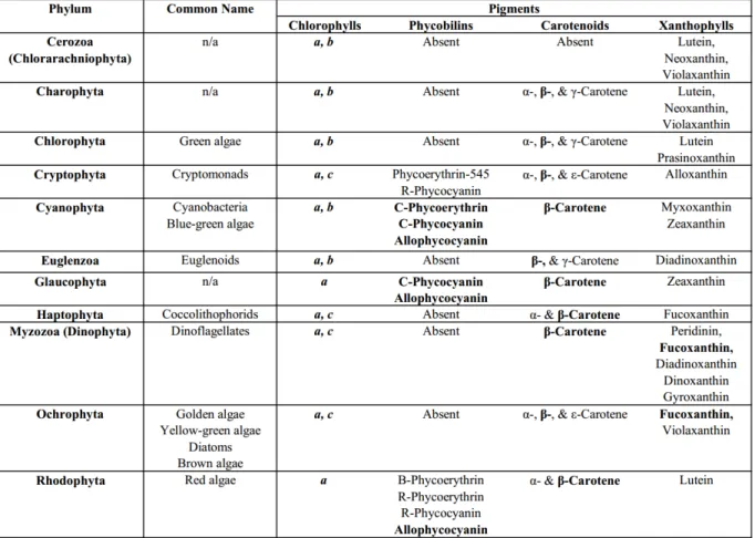
3.1 Different phlya of algae contain different pigments within their structure. The most noticeably pigments are the Chlorophylls, C-Phycoerythrin (C-PE), C-Phycocyanin (C-PC), and allophycocyanin (APC) [21]. . . 12

5.1 The 12 models that will be evaluated side-by-side result from three set of options when building a model. The first option is: which data do we use? The second options is: how do we represent that data? And the third option is: how does that data propagate through the network? . . . 58

7.1 The classification accuracy is reported for the train, validation, and test sets when evaluating the 12 proposed software frameworks. . . 81

7.2 A T-Test between two consecutive models was run where the only difference in the models is the use of a flat structure as opposed to a hierarchical struc-ture. For a p-value of 0.01 there was no noticeable improvement between any of the models. For a p-value of 0.05 only one model showed a statically significant decrease in performance when using a hierarchical approach. . . 84

7.3 A further breakdown of the 12 model architectures reveals how the accuracy of the model throughout the three levels of the tree. . . 86

(19)

Chapter 1 Introduction

“Access to water is access to education, work, and the kind of future we want for all the members of our human family.”

– Co-founder of water.org, Matt Damon (1970 - present)

This introductory chapter provides the reader with a high level overview of the entire thesis. First, in Section 1.1, an overview of harmful algae blooms (HABs) will be given. Then, in Section 1.2, the problem of manual identification of algae will be discussed. Finally, in Section1.3, the main scientific contributions and outline of the thesis will be presented.

1.1 Motivation

We live in an amazing time. In general, people are living healthier and longer lives due to advances in medicine and health. Thanks to modern transportation one can now travel anywhere in the world. And thanks to the digital age, we can communicate with anyone from nearly anywhere on the planet. Despite these optimistic observations, the world still has significant concerns. These include, but are not limited to: poverty, lack of access to clean drinking water and basic education, human sex trafficking, gender inequality, our rapid energy consumption, and climate change. In fact, in 2015 the United Nations (UN) created the Sustainable Development Goals outlining 17 major goals which they hope to reach in the near future [1]. The 150 targets included in these goals were proposed by sector experts.

(20)

Figure 1.1: The Moderate Resolution Imaging Spectroradiometer (MODIS) on the Aqua satellite showing a harmful algae bloom (HAB) on Lake Erie on October 9, 2011 [2].

However, this overwhelming amount of targets created its own problems. How are the targets prioritized? Which of these problems are actually solvable given our current technologies, resources and time frame? Bjorn Lomborg, who led a team of economists, set out to answer these questions and took on the task of prioritizing and ranking the order of the UN targets. Lomborg explains that while these targets are commendable, many are also unrealistic and unpractical. He argues that by pursuing unachievable goals, we will actually hinder our progress instead of advancing it. For these reasons Lomborg and his team proposed a set of 19 achievable targets, resulting in the greatest return on every dollar spent on a given problem [3].

In the spirit of tackling a major world problem as proposed by the UN, while honouring the focus on urgent problems as identified by Bjorn Lomborg, this thesis will make a con-tribution to the challenge of providing clean water to all regions of the earth. The specific focus of this thesis is the identification of algae in water with the goal of more efficient management of harmful algae blooms (HABs). Recently, harmful algae blooms (HABs) have become a common experience around the globe. For example, as seen in Figure1.1, in the summer of 2011 Lake Erie experienced a severe harmful algae bloom [4]. According to the Great Lakes Environmental Research Laboratory this bloom was primarilyMicrocystis aeruginosa, a type of lethal cyanobacteria [2].

(21)

swallowing Microcystis can lead to serious reactions, such as abdominal pain, diarrhea, vomiting, blistered mouths, dry coughs, and headaches. In addition, Anabaena, another common cyanobacteria, can produce lethal neurotoxins called anatoxin-a which are shown to have caused death by progressive respiratory paralysis [5]. Therefore it is essential for the proper management of any water that the water quality is monitored for different cyanobacteria and other algae [6]. The preservation and maintenance of our water directly affects marine wildlife, as well as the recreational, fishing and tourism industries. Moreover, water maintenance is crucial for water treatments plants that are in charge of distributing clean drinking water to the population.

However, as we will see in Section 1.2, this poses a significant problem as samples of water must be taken from the source of water and shipped to a certified laboratory for inspection. Then these samples must be manually inspected under traditional microscopy techniques and each algae type is manually identified and enumerated.

1.2 Overview of Problem

The current method to monitor algae requires a human expert, a taxonomist to use a microscope in order to manually identify and enumerate each algae. Due to the low number of algae taxonomists available and the extensive experience required to classify different algae, the process to identify and enumerate algae is time-consuming [6].

In addition, since the sample must travel to the taxonomist, there is additional transit time, which further increases the turn-around time and the cost of analysis. Due to this long process it is nearly impossible to maintain ongoing active monitoring of a given water body for different algae and cyanobacteria [7,8]. To understand the environmental precursors to algae blooms, and to study the behaviour of algae under different environmental factors, a in-situ method to quantitatively identify and measure different algae species is essential and much needed [8].

The problem that will be addressed and solved in this thesis is the need for human ex-perts to manually identify different types of algae by looking through a microscope. This problem will be solved by creating a novel imaging system that using machine learning methods to automatically identify different types of algae in water samples. Solving the problem of manual identification removes the need to transport the sample away from the source water, removing the burden of analyzing back-logged samples by trained tax-onomists. Therefore this thesis provides a method for on-site analysis of water samples which can be analyzed in real-time using machine learning models.

(22)

Figure 1.2: This thesis is composed of 8 main chapters. After this introductory Chapter1, Chapter 2goes into detail of the background of HABs and algae, while Chapter 3 present the current methods of automatic identification of algae. Chapter4presents the hardware contribution of this thesis and Chapter 5 describes the software framework. Then, in Chapter 6 a dataset is created in order to evaluate the efficacy of the Contribution 1 and Contribution 2. In Chapter 7 the results are presented and in Chapter 8 the final conclusions are discussed.

(23)

1.3 Thesis Contributions & Outline

Given the importance of identifying algae and the current limitations of the manual pro-cess, this thesis proposes a new method to automatically identify algae in water. This work is broken in eight chapters, as seen in Figure1.2. After this introductory chapter, Chapter

2 will go into further details of HABs and the current practices of manual identification. Chapter2extensively covers the problem being solved in this thesis. We will see how man-ual identification and enumeration using a microscope is both tedious and time-consuming, and is very prone to human bias and error.

As discussed by Walkeret al., developing a method to automatically identify algae down the genus or species level using modern imaging systems in combination with pattern recognition techniques would be extremely valuable [8]. Sieracki et al. add that these systems can potentially be used as an early warning sign for harmful algae blooms in water bodies since these imaging systems can record the contents of predetermined water volumes at high rates [9]. Therefore, in Chapter 3, the various methods to automate the identification of algae will be presented. These methods include digital microscopy, imaging flow cytometry, spectral analysis, fluorescence probes, and genomics.

To date, each method discussed in Chapter3has been fairly independent from the other. Therefore, the proposed research combines two of these methods, the spatial element from digital microscopy with the spectral element of fluorescent spectroscopy. The proposed solution has three main scientific contributions, which are presented in the next three chapters:

1. Contribution 1: Creation of a novel imaging device for low-cost acquisition of ab-sorption and multispectral fluorescence images of algae (Chapter 4).

2. Contribution 2: Creation of a software framework to automatically identify algae using multispectral-based classification & taxonomy-based-hierarchical classification (Chapter 5).

3. Contribution 3: Creation of a novel dataset using Contribution 1 in order to test Contribution 2 (Chapter 6).

Given this dataset, Chapter 7will present the relative performance of all these models and highlight the use-case for each one in order to determine the efficacy of Contribution 1 and Contribution 2. Finally in Chapter 8, the main conclusions and future work will be presented.

(24)

Chapter 2 Problem

“In the year 1657 I discovered very small living creatures in rain water.” – ‘the Father of Microbiology’, Antonie van Leeuwenhoek (1632 – 1723)

After the brief description of the problem in Chapter 1, this chapter presents further details of HABs in Section 2.1 and the process of manual identification of algae in Section

2.2. We will see that it is imperative that drinking water treatment plants closely monitor algae as this can be an indicator to assess which toxins are present in their source water. Furthermore, we will examine why the current method of manual identification is time-consuming and tedious.

2.1 Harmful Algae Blooms (HABs)

Harmful algae blooms (HABs) develop when different types of algae grow out of control in a water body causing them to produce lethal toxins. HABs are happening all around the world, from the North American Great Lakes, to the African Great Lakes and from Lake Taihu in China to the Baltic Sea [12]. These HABs are having severe global economic and social impact as they are affecting drinking water quality, recreational use of water and tourism, as well as the fishing industry [13]. For example, during the 2014 Toledo water crisis over 400,000 people lost access to clean drinking water for nearly three days [14].

(25)

Table 2.1: The State of Ohio presents the common algae which are known to produce different toxins [10]. Knowing whether toxic producing algae are in a water body is critical information for a drinking water treatment plant [11].

Furthermore, the number of blooms being observed has been increasing rapidly [15], and due to phosphorus and nitrogen runoff in combination with climate change these blooms are only expected to increase in severity. [12, 16].

One common toxin produced by a number of algae is known as microcystin, as seen in Table 2.1. This toxin has a threshold guideline set by the World Health Organization (WHO) since it is lethal for humans [17]. The maximum acceptable concentration (MAC) for the cyanobacteria toxin microcystin-LR in drinking water is 1.5µg/L, according to the Government of Canada [18, 11]. In addition, in 2014 the U.S.A. released the Harmful Algal Bloom and Hypoxia Research and Control Amendments Act (HABHRCA), which requires the National Oceanic and Atmospheric Administration (NOAA) and United States Environmental Protection Agency (USEPA) to advance the scientific understanding and ability to detect, monitor, assess, and predict HABs and hypoxia events in marine and freshwater in the United States [19].

Many different algae are the source of different toxins in our drinking water, as seen in Table2.1, which is presented by the State of Ohio [10]. Therefore knowing which algae are

(26)

present in a water sample provides insight into whether an algae bloom will have toxins or not. To quote the Ohio State EPA:

“Phytoplankton samples can be collected to determine the cause of the bloom. If cyanobacteria are present, the manager should use [Table2.1] ... to determine if the bloom is capable of producing cyanotoxins, and which cyanotoxins should be analyzed.”[10]

Health Canada also voices the need for accurate counts which are provided by a highly trained professional:

“The use of a trained microscopist with experience in identifying cyanobacteria is favourable when performing cell counts.”[11]

2.2 Manual Algae Identification

Given the importance of having a trained professional with the ability to identify different algae, it is worthwhile to understand this history and current practices of trained tax-onomists. As explained by He et al., the WHO also suggests to use cyanobacteria and algae identification and enumeration by a human expert as a screening tool to asses the severity of an algae bloom. However, this process requires a high level of expertise as well as time and for that reason becomes unsuitable as an early warning sign [20].

As seen in Figure 2.1, the standard method of identifying and enumerating microalgae consists of three main steps which are: (1) sample preparation, (2) classification, and (3) enumerating. The purpose of the sample preparing is to condense the algae down to a higher concentration that can then be observed. The three main methods to condense the sample are filtration, centrifugation and use of sedimentation. Identification of different genera and species is done manually by the human taxonomist. Lastly, a counting chamber is used to aid the taxonomist in enumerating the sample. Before analysis of the sample can occur the sample must first be concentrated. The two methods to concentrate live samples are filtration and centrifugation, while sedimentation is used for preserved samples. In general, centrifugation and sedimentation are the most common depending on whether the cells are alive or are being preserved, however filtration is an effective means as well [21].

When identifying unicell or small colonies by way of filtration or centrifugation, counting chambers such as the haemacytomter, the Thoma chamber, the Fuchs-Rosenthal or the Burker chambers can be utilized to estimate the density of a variety of cultures. All these

(27)

Figure 2.1: The standard method of identifying and enumerating microalgae consists of three main steps which are: (1) sample preparation, (2) classification, and (3) enumerating. The three main methods to condense the sample are filtration, using centrifugation and sedimentation [21].

chambers have a grid with known spacing in order to determine the different microalgae counts. In addition, most of these cell counters have very delicate surfaces that cannot be scratched and must be handled very carefully [21]. When using sedimentation a special type of counting chamber known as an Uterm¨ohl chamber can be used to identify and count different microalage. These Uterm¨ohl chambers are usually very expensive and also require time (approximately one day) to settle to the bottom of a solution. Furthermore, a solution is added to the sample that kills and preserves the sample, which allows them to sink to the bottom of the solution on account of gravity. The advantage is that now the sample can be directly placed on an inverted microscope which can be used to observe random sections of the condensed algae which facilitates the identification and enumeration of microalgae [21].

Throughout the history of phycology, the study of algae, considerable effort was put forth to classify and organize the diversity of algae into distinct groups. However little effort was made to provide “identification (ID) keys” in order to facilitate its usefulness to others, until 1931 when Lily Newton published her handbook of algae in the British Isles [22]. 31 years later, in 1962, Eifion William Jones published his key to the genera

(28)

Figure 2.2: Manual identification of algae requires a human expert, a taxonomist, to manually look through a microscope and classify all the organisms present in a water sample. This method requires years of experience and is both time-consuming and tedious. of British seaweed [23]. Throughout the last 50 years many others have released keys in form of books [24, 25]. Since the advent of the internet numerous credible sources have released online ID keys providing images of algae under a microscope to assist both novice and professional taxonomists [26,27, 28].

Regardless of what key taxonomists use, they must observe the algae under a micro-scope, and compare their observations against the ID key, as seen in Figure2.2. Constantly switching between between these two tasks is tedious, time consuming [29], and may cause straining on the eyes. A study by Culverhouse et al. estimate that human taxonomists have a self-consistency identification accuracy between 67% to 83% and a 43% consensus when comparing between taxonomists [30]. Furthermore, as identification can take hours the taxonomist will likely fatigue, increasing the likelihood of a miss-classification. Due to this time-consuming process the average time it takes for a given organization to get the taxa breakdown of a water sample can be anywhere from a few days to a week. It is for these reasons that many people have explored the automation of this task using digital imaging and pattern recognition, as will be discussed in Chapter 3.

(29)

Chapter 3 State of the Art

“If I have seen further it is by standing on the shoulders of giants.” – Sir Isaac Newton (1643 - 1727)

Over the years there have been many different methods to automatically identify algae. First off, in order to get an understanding of the biological classification of algae, an overview of algae taxonomy and pigmentation will be presented in Section 3.1. We will see that different algae groups have different associated pigments, and that these pigments also have different spectral absorption curves.

Next the automated methods will be presented. In this thesis these methods will be grouped into five main categories: microscopy based methods (Section 3.2), imaging flow cytometry based methods (Section3.3), spectral based methods (Section 3.4), fluorescence probe based methods (Section 3.5), and finally genomics based methods (Section 3.6).

Microscopy methods can be further broken down into brightfield microscopy (Section

3.2.1), fluorescence microscopy (Section3.2.2), and a combination of brightfield and fluo-rescence microscopy (Section3.2.3). Spectral methods remove any spatial components and consist of absorption spectroscopy (Section 3.4.1) and fluorescence spectroscopy (Section

3.4.2). After exploring these methods a summary of the main findings for each method will be presented in Section3.7.

(30)

3.1 Algae Taxonomy & Pigmentation

The term algae has no clear definition since many organisms that are referred to as algae come from significantly different branches in the tree of life. For example, cyanobacteria (blue-green algae) belong to the bacteria domain, while green algae belong to the eukarya domain. The domain division is the lowest base rank split in the taxonomic structure, illustrating that the term “algae” can include significantly different organisms. The one characteristic of all algae is that they have chlorophyll and occasionally other pigments to carry out photosynthesis. Using pigmentation to classify different algae was first done by William Henry Harvey in 1836 when he divided algae into four major divisions:

Rho-Table 3.1: Different phlya of algae contain different pigments within their structure. The most noticeably pigments are the Chlorophylls, C-Phycoerythrin (C-PE), C-Phycocyanin (C-PC), and allophycocyanin (APC) [21].

(31)

dospermae (red algae), Melanospermae (brown algae), Chlorospermae (green algae) and Diatomaceae (diatoms) [31].

As provided by Barsanti et al. [21], a common and modern classification of algae into different groups can be seen in Table 3.1. This classification scheme groups algae into different phylum groups, as seen on the left in Table 3.1. Cyanophyta, as previously mentioned in Chapter1and Chapter2, are commonly known as cyanobacteria or blue-green algae, and is the group of algae that is most associated with harmful algae blooms. Other common phyla groups are Chlorophyta (commonly known as green algae), Euglenzoa, dinoflagellates, as well as diatoms and red algae.

Table 3.1 also highlights the major pigments present in each phyla group. While all algae contain chlorophylls, certain algae groups contain specific pigments that other groups do not have. For instance, Cyanophyta have three common phycobilin pigments, C-Phycoerythrin (C-PE), C-Phycocyanin (C-PC), and allophycocyanin (APC), while these phycobilin pigments are completely absent from Chlorophyta, Euglenzoa and other phyla groups. A similar pattern can be observed when inspecting the carotenoid pigments and the xanthophyll pigments. For example, Cyanophyta only containsβ-Carotene, while other groups contain additional carotenoid pigments. The other important thing to consider is that even if two phyla groups have the same pigments present, they likely have different concentrations of that pigment. For example, while both Cyanophyta and Chlorophyta contain chlorophyll-a, one phyla may have more of that specific pigment than the other. As we will see later in Chapter 6, this in fact can be observed.

As one may expect, each pigment has a different associated spectral curve that occupies a unique part of the electromagnetic spectrum. This is illustrated in Figure 3.1, where we see seven common pigments that were reported by Coltelli et al. [32]. Inspecting the spectral absorption curves reveals that chlorophyll-a and chlorophyll-b have peaks in the blue part of the spectrum (400 nm - 475 nm) as well as in the orange and red part of the spectrum (600 nm - 700 nm). This is opposed to B-Phycoerythrin (B-PE) that occupies the green part of the spectrum (500 nm - 600 nm) and C-Phycocyanin (C-PC) which occupies the orange part of the spectrum (550 nm - 650 nm).

Since different pigments have unique spectra, and since different algae phylum groups have different combinations of pigments, one can deduce that a given algae group will likely have a unique spectrum relative to another algae group. As we will see in Chapter

3, this reality is commonly used in spectral methods (Section 3.4), however, is it rarely used in combination with digital microscopy (Section 3.2). Only a few researchers have explored leveraging both the spectral uniqueness of algae due to their pigments and the spatial uniqueness of algae due to their different morphologies (Section 3.2.3).

(32)

Figure 3.1: As observed in Table 3.1, different phyla of algae contain different antenna pigments [21]. Here the major pigments are shown on a single plot [32]. Note how different pigment are spread across different parts of the visible spectrum.

3.2 Microscopy Methods

A microscope is an optical device that magnifies a given sample by orders of magnitude in order to viewed by human eyes or a digital sensor. Two common forms of microscopy are known as brightfield microscopy (Section 3.2.1) and epi-fluorescence microscopy (Sec-tion 3.2.2). Newer methods have been combining both brightfield and fluorescence mi-croscopy (Section 3.2.3) as research has shown that a combination of this data allows for higher performance when classifying organisms. By attaching a digital camera to either of these microscope systems, one can capture one or more digital images which can be used as input into a pattern recognition algorithm. The majority of the related work surrounding automatic identification of algae uses feature extraction methods where distinct descriptors are measured from a given image and then inputted into a machine learning algorithm such as a support vector machine or decision tree.

3.2.1 Brightfield Digital Microscopy

Brightfield microscopy is an imaging modality where a broad band light source is placed below the sample in order to illuminate it. Then a set of objective lenses are placed above

(33)

the same which focus the light into an eyepiece for viewing by a human, or onto a camera sensor for capturing a digital image. Brightfield microscopy is the most elementary and low-cost forms of microscopy [33]. Early work on automatic algae classification began in 1995 when Thiel et al. collected brightfield images of nine genera of blue-green algae and two genera of green algae, used 14 Fourier descriptors, 6 cell features, 7 moment invariants and 20 statistical features for texture, and used discriminant analysis to build a classifier [7]. They achieved 98.10% accuracy when classifying from these 11 different genera when training and testing on 158 samples. However, due to the small dataset and the omission of evaluating their discriminant classifier with a test set, the results likely showed an overfitted model to the training data.

Major work was done by Walker et al. in 2000 when they used a multiclass hierar-chical classifier structure to properly classify four different species of Anabaena and two different species of Microcystis [8]. They measured 123 object features, including morpho-metric properties, object boundary shape properties, frequency domain properties, and second-order statistical properties and then used stepwise regression to find discriminatory features. Using a general Bayes decision function they achieved 97% accuracy when clas-sifying. Although they only used cultured cyanobacteria, their work has shown that when enough data is present classifying multiple species is relatively accurate. In 2014, Promdaen et al. [34] developed a method to classify 12 different genera of microalgae with 97.22% classification accuracy, using data collected from a variety of brightfield microscopes. These genera included three types of toxic blue-green algae(Anabaena, Oscillatoria, Microcystis) as well as 7 genera of green algae, and one genus of Euglenoids. Feature extraction involved using Fourier descriptors, moment invariants, shape measures and texture features, while their classifier was a support vector machine.

Next, Coltelli et al. released a paper in 2014 in which they describe how they used a self-organizing map (SOM), an unsupervised learning method, to achieve 98.6% accuracy from a set of 53,869 images of 23 different microalgae representing the major algal phyla [6]. After acquiring the images and segmenting the algae, the RGB images were converted to the L*c*h* color space (lightness, chroma, and hue) and the morphological features were extracted. To recognize the different algae, these features were grouped into classes using clustering. Very recently, in 2019 Iamsiri et al. [35] used three geometric shape features (solidity, eccentricity, and convexity) as well as 13 features derived from a gray level co-occurrence matrix (GLCM) to train a support vector machine and achieve a classification accuracy of 91.30%. This was achieved while classifying five filamentous types of algae: Anabaena, Oscillatoria, Spirogyra,Spirulina, and Anabaenopsis.

Overall, supervised learning methods such as support vector machines (SVMs), naive Bayes, decision trees, and k-nearest neighbour have all been utilized to learn the optimal

(34)

classifiers for different genera of microalgae when imaged under brightfield microscopy. As inputs to these models the features used are primarily morphometric properties (diameter, area, convex perimeter, elongation, etc.), but also Fourier descriptors, moment invariants, and statistical texture features. It is important to note that all these methods are tra-ditional feature extraction methods and do not leverage feature learning capabilities. In addition, active learning and unsupervised learning methods have also been utilized and have shown to be effective means of classification of different types of microalgae. There-fore brightfield microscopy coupled with different classifiers is a viable method to classify different types of cyanobacteria both to the genus level [7, 34, 6, 35], as well as to the species level [8].

3.2.2 Fluorescence Digital Microscopy

The most widely used form of fluorescence microscopy is known as epi-fluorescence mi-croscopy, which was invented by Johan Sebastiaan Ploem (1927 - present) [36]. In this image modality a broadband light source, usually a mercury arc lamp, emits high energy light into a filter cube. The light entering the filter cube passes through an excitation filter which selects a narrow band of light which will reflect off a dichroic mirror and then fo-cused onto to the sample using the objective lens. This high energy light causes the sample to fluorescence, resulting in lower energy light being emitted from the sample. This lower energy light passes through the objective lens and into the filter cube. Given the properties of the dichroic mirror, the low energy light passes through the dichroic mirror, and then is filtered by an emission highpass filter. Finally, this emission signal is then focused into an eyepiece for viewing by a human or onto a camera sensor in order to capture an image.

In 2006 Ernst et al. [37] developed an automated system to count filamentous Plank-tothrix rubescens using image processing. By using a single band epi-fluorescence setup they were able to identify and estimate the cell density for three different environmental samples and one cultured sample of Planktothrix rubescens. They found that the Plank-tothrix rubescens could be easily separated from algae when imaging under a fluorescence setup.

In 2016 Jinet al. used fluorescence microscopy to separate Microcystis aeruginosa [38] andAnabaena flos-aquae[39] from the background by exciting the respective samples at 546 nm and leveraging a Maximum Likelihood (ML) classifier. In both papers, Jinet al. then enumerated the samples and calculated size statistics. When comparing their results to the manual enumeration data using an hemacytometer they found their method achieved higher accuracy using much less time and resources. These papers [38,39] illustrate the power of

(35)

using the auto-fluorescence of cyanobacteria to separate the cyanobacteria samples from the background. However, these methods only inspect a single species of cyanobacteria at a single fluorescence wavelength and do not explore using multi-band fluorescence microscopy to classify between different genus or species of cyanobacteria and other microalgae.

3.2.3 Brightfield & Fluorescence Digital Microscopy

As we have seen, both brightfield microscopy and fluorescence microscopy can be used to classify different genera of microalgae. However, when combining these two modalities we have the potential to improve our classification capabilities.

In 2006 Rodenacker et al. [40] developed a system called PLASA (Plankton Structure Analysis) that captured four fluorescence images and a brightfield image by using two flu-orescent filters in tandem with a RGB camera. The first fluflu-orescent filter cube had an excitation of 450 nm - 490 nm with a emission long pass filter of 515 nm. The second fluorescent filter cube had an excitation wavelength of 546 nm with a bandpass filter of 600 nm ± 40 nm. They also developed a segmentation system which fed into a feature extraction system in order to automatically identify different algae types. Henseet al. pub-lished a paper in 2006 using the PLASA system [40] which allowed for both bright-field and fluorescence images to be captured. They showed that autofluorescence information improves the discrimination between algae and non-algal objects and also distinguished between phycoerythrin (PE) containing algae and other algae [41]. One of the few im-portant insights learned from Hense et al. is that thresholds based on fluorescent ratios opposed to fluorescent intensities proved more effective for discriminating between algae vs non-algae objects. In addition, they observed that under repeated excitation, chlorophyll-a and phycoerythrin emission intensity show an exponential decay, which they call fluores-cent fading. In order to combat this fluoresfluores-cent fading, appropriate image acquisition is required. Overall they found that the main benefit of using fluorescent information was the separation of algae species from non-algae species and large amounts of detritus; therefore Hense et al. recommend using multiple fluorescent features.

Walker et al. came to the similar conclusion that if accurate species level classifica-tion is required, it is necessary to capture both fluorescence and brightfield images [42]. Therefore, in 2002, Walkeret al. illustrated that by capturing a single fluorescence image and a single brightfield image over 97% classification accuracy is possible when looking for Anabaena sp. and Microcystis sp. in natural populations found in Lake Biwa, Japan [42]. Without the use of fluorescence imaging the automated analysis of microalgae in the sedi-ment saturated samples is nearly impossible. In order to achieve this high accuracy they

(36)

accomplished image registration using template matching and region growing techniques. As a result 120 different features (morphometric, boundary shape, frequency domain, and second-order statistics) were found and used to build a general Bayes decision function with Gaussian distributions. However, they acknowledge that due to current hardware limitations this is not viable, and therefore they limited their research to a single fluores-cence image and a single brightfield image. Walkeret al. believe that future improvements in fluorescence imaging will enable a low-cost, automated, species-level analysis and clas-sification of microalgae. In addition, they only explored a traditional feature extraction based method and they did not leverage modern feature learning methods such a deep neural networks.

3.3 Imaging Flow Cytometry

Imaging flow cytometry takes an existing microscope system and incorporates a flow sys-tem in order to increase the throughput of the syssys-tem. This imaging flow cytometry is a hybrid of the speed and statistical capabilities of flow systems, combined with the imaging feature of digital microscopy [43]. This allows for more samples to be collected, resulting in a more representative distribution of a given algae population. Some common, commer-cially available imaging flow cytometry systems built for automated algae analysis are the Cytobuoy, the Flow Cytometer And Microscope (FlowCam) by Fluid Imaging Technolo-gies, and the Imaging FlowCytobot (IFCB) by McLane Labs. As we will see, these flow systems are often acquired by research labs to investigate the efficacy of such a system to collect unique data which can be used in a machine learning model. Several important studies related to the automatic identification of algae using imaging flow cytometry are highlighted below.

Blaschko et al. conducted a thorough investigation using 982 images of 13 different classes of plankton collected from a FlowCAM device in 2005 [44]. They used five different groups of features which were simple shape, moments, contour representations, differential and texture features. They then evaluated the classification performance using the fol-lowing algorithms: decision trees, naive Bayes, ridge regression, k-nearest neighbour, and support vector machines. In the end the best classifier, a SVM, was able to achieve only 71.08% accuracy.

In 2007 Heidi M. Sosik created the Imaging FlowCytobot (IFCB) to explore automatic classification of phytoplankton [45]. In this study the submersible device collected images which were used to extract features (size, shape, symmetry, texture, invariant moments, and co-occurrence matrix statistics) to be entered into a machine learning algorithm. They

(37)

trained and tested a 22 category classifier which achieved 88% overall accuracy. This rev-olutionary technology allowed an unbiased approach to classify large amounts of phyto-plankton data.

In 2013, Colares et al. used active learning in order to boost the performance of a classifier from microalgae data which were captured using a FlowCAM system [46]. The FlowCAM system provided 26 different features to represent the data, however Colareset al. only used seven of those features from two datasets. The first dataset contained 1,526 images consisting of four classes: Flagellates (1,003 images), others (500 images), pennate diatoms (14 images) and mesopores (9 images). The second dataset is composed by 923 images consisting of four classes: Pennate Diatoms (112 images), Flagellates (669 images), gymnodinium (65 images) and prorocentrales (77 images). Two metrics, accuracy and maxF1, were used to evaluate the performance of their approach and their final Gaussian mixture model with expectation-maximization classifier had an accuracy of 92%.

In 2016, Corrˆea et al. used supervised learning on FlowCAM data which consisted on an imbalanced dataset of 24 types of microalgae divided in 19 classes [47]. They used the Synthetic Minority Oversampling Technique (SMOTE) to achieve oversampling strategy to compensate for the imbalances of their data. They evaluated five different supervised classification schemes which included multilayer perceptrons, the naive Bayes classifier, decision trees, and k-nearest neighbour (kNN). The input to these classifiers were ten manually-chosen features selected from the FlowCAM data. Three metrics were evaluated to produce the results which where Kappa, MaxF1 and MinF1. The best performance classifier was a kNN and has the scores of 98.1%, 98.2%, and 98.2% for Kappa, MaxF1 and MinF1 respectively.

Newer methods of imaging flow cytometry are beginning to use deep learning models to automatically identify algae. In 2018, Göröcs et al. [48] used a deep learning approach with a portable imaging flow cytometer in natural water samples. They captured diffraction patterns of flowing microorganisms and then use object detection and deep learning-based hologram reconstruction. They used this device for the detection of microplankton and nanoplankton ocean in samples along the Los Angeles coastline. By combining the ability of computational algorithms with deep learning Göröcs et al. were able to create a cost-effective, high-throughput flow cytometer to monitor algae.

3.4 Spectral Methods

Having covered the microscopy based approaches we will now shift to systems that have no spatial component, but only a spectral component in the data. Spectral based methods

(38)

Figure 3.2: The absorption of light of a solution can be measured by passing a known broadband light source through the solution and measuring the transmitted signal with a spectrometer.

can be further broken down into absorption spectroscopy methods (Section 3.4.1) and fluorescent spectroscopy methods (Section3.4.2). A spectrometer is a device that has the ability to measure the relative intensity of different wavelengths across the electromagnetic spectrum. Since the light-matter interaction is unique for different substances, light will reflect, absorb, fluoresce and transmit at different intensities for different wavelengths. Spectral methods are most accurate when the sample is assumed to be homogeneous: care is taken that only one type of algae is present. Due to spectral mixing, which occurs when different algae are present in the same sample, the spectrum of each is combined into a single signal, making it difficult to determine the relative amount of each organism.

3.4.1 Absorption Spectroscopy

As seen in figure 3.2, the absorption spectra of a solution can be measured by passing a known light source through a sample, and then measuring the transmitted light by a spectrometer. The absorbance of a material, denoted by A is defined as:

A=log10Φi Φt

=−log10T, (3.1)

where, Φi is the radiant flux incident on the material, Φt is the radiant flux transmitted

(39)

Figure 3.3: The absorption of algae for different phyla groups reported by Lee et al. (top) [49] and Held et al. (bottom) [50].

The absorption of different algae, as seen in Figure 3.3, has been described in two papers. The first paper is by Lee et al., who in 1994 measured three algae, each from a different phyla group [49] from 400 nm - 750 nm. These algae were from the Cyanophyta phylum, Chlorophyta phylum and the Dinophyta phylum. As seen from Figure 3.3 all three algae peaked in the 400 nm - 475 nm range as well as in the 650 nm - 725 nm range. The Cyanophyta also had a peak in the 575 nm - 650 nm range These spectral responses all match the pigmentation data presented earlier in Table 3.1 as only Cyanophyta are reported to have phycobilin pigments.

(40)

Figure 3.4: A fluorescence spectra can be measured by using a broadband light source which passes through a narrow bandpass filter to isolate the excitation wavelengths. This excitation light enters the sample, causes the sample to fluoresce, and emits a lower energy light signal. This lower energy light gets filtered by an additional highpass filter and then measured by a spectrometer.

2011 [50]. This spectrum was measured from 300 nm - 700 nm and has similar trends as the data reported by Lee et al. [49], but with a slightly different ratio of peaks. It is also interesting to observe the strong absorption of this algae in the ultraviolet part of the electromagnetic spectrum.

These spectra show that there is the potential to discriminate between different algae phyla groups when using absorption spectra methods. However, as seen in Section 3.4.2, most methods of spectroscopy use fluorescence based methods, where the excitation and emission spectra of different algae tend to range much more than the absorption spectra of different algae.

3.4.2 Fluorescence Spectroscopy

As seen in Figure3.4, fluorescence spectroscopy involves using a light source and a narrow bandpass filter to excite a sample at a high energy, corresponding to a lower wavelength and then measuring the emission spectra at a lower energy, using a highpass filter, as seen in Figure3.4. The excitation wavelength excites the sample by absorbing a photon of light and causes an electron to jump in energy state. When this electron then falls from this higher

(41)

Figure 3.5: The excitation spectra from 400 nm - 650 nm was reported by Poryvkinaet al. [51] (top) and Gsponer et al. [52] (bottom). These spectra reveal significant differences in the excitation wavelengths for different phyla of algae.

state, the energy is emitted as light at a higher wavelength. This is, in fact, the same technique that epi-fluorescence methods (Section 3.2.2) use. Since fluorescence spectra have both an excitation and corresponding emission spectra, both will be discussed. Some papers only present either the excitation or emission spectra while others present both.

(42)

Excitation Spectra

Poryvkinaet al.[51] measured the excitation spectra of 31 algae species from seven phyla. In Figure 3.5 (top), four of the 31 excitation spectra can be seen from two of the phyla (Chlorophyta, Cyanophyta). In addition, Gsponeret al.[52] measured the norm excitation spectra of five algae species from four phyla (Chlorophyta, Rhodophyta, Cyanophyta, and Dinophyta) as seen in Figure3.5(bottom). Both of these studies [51,52] demonstrate that different algae types have unique fluorescence excitation spectra from each other caused by the difference in pigments in a given algae type, as well the relative concentration of a given pigment, once again matching the different pigments from Table3.1.

Another very interesting observation from Figure 3.5 is that excitation spectra differ significantly compared to the absorption spectra seen in Figure 3.3. This reveals the potential use of fluorescence data as a method to achieve high separability as well as a method of classifying different algae types. In fact, we will leverage this information when designing our own hardware system in Chapter4and then report the corresponding classification accuracy of using only fluorescence spectra in Chapter 7.

Emission Spectra

To determine this we must first look at work previously published by Frenchet al.[53] and Millie et al. [54] as seen in Figure 3.6.

French et al. [53], as seen in Figure 3.6 (top), measured the emission spectra of Por-phyridium cruentum, a type of red algae, from 570 nm - 750 nm when exciting the sus-pended sample at 11 different narrow-band wavelengths from 405 nm - 546 nm by using a high pressure mercury lamp and additional optics. Figure 3.6 (top) illustrates that when plotting three of the eleven emission curves the fluorescence emission increases when going from 490 nm to 515 nm to 546 nm. In fact, this matches the work presented by Gsponer et al.[52], whose data can be seen in Figure 3.5 (bottom), since the only species from the Rhodophyta phyla peaks around 550 nm.

Millieet al.[54]. excited five different samples of microalgae from four different phyla at either 440 nm or 490 nm. In Figure3.6 (bottom), four samples, from three different phyla, are presented, where the spectra were normalized to a range of zero and one. Each of these fluorescence emission spectra from the presented three phyla (Cyanophyta, Dinophyta, and Chlorophyta) are relatively unique as they each have a distinct peak wavelength. Therefore, as expected, the emission spectra for different phyla are relatively unique which is caused by the distinct pigments in each phyla as previously shown in Table3.1. Furthermore, this information can be leveraged when designing and building an imaging system.

(43)

Figure 3.6: The emission spectra of Porphyridium sp. by French et al. [53] (top) and the emission spectral of four common algae from three phyla groups by Millieet al. [54]. These spectra show that different algae have different emission spectra which is the result of these algae having different different pigments. Notice the wavelength range in this figure compared to the wavelength range in Figure 3.5. Since the emission spectra is at a lower energy, the spectra will be at a higher wavelength.

In addition to measuring the excitation spectra of five different types of algae, Gsponer et al. [52] took one sample (Microcystis sp.) and also measured the emission spectra. As seen in Figure 3.5 (bottom) and Figure 3.7, Microcystis sp. has a peak excitation wavelength between 600 nm and 625 nm. As seen in Figure 3.7, the corresponding peak emission wavelength is approximately 680 nm.

(44)

Figure 3.7: The excitation and emission spectra ofMicrocystis sp. measured by Gsponeret al. (top) [52] and by Heldet al. (bottom) [50]. While the emission spectra is very similar, the excitation spectra varies between these two authors.

In addition to these reports about excitation and emission spectra, work has been done in exploring a fluorescence-based approach to identifying algae. In 2002, Beutler et al. built a custom device that used five distinct wavelength LEDs (450 nm, 525 nm, 570 nm, 590 nm, and 610 nm) to excite different pigments in five different algae spectral groups, which were: green algae (Chlorophyta), glue-green algae (Cyanobacteria), brown algae (Bacillariophyceae and Dinophyceae) and mixed algae (Cryptophyceae). These LEDs excited the Chlorophylla pigments as well as other antenna pigments such as Chlorophyllc, phycocyanobilin, phycoerythrobilin, fucoxanthin and peridinin [55]. By placing a bandpass filter between the algae sample and the sensor they were able to take five measurements