Development of Novel Methods of
Analysis for Indoor Air Pollutants
Chunting Michelle Wang
Doctor of Philosophy
University of York
Chemistry April 2017ii
Abstract
The current variability and speciation of indoor VOCs are studied by analysing indoor air in UK homes and offices. These measurements were carried out via passive sampling into silica-treated canisters followed by thermal desorption-gas chromatography and high mass accuracy time-of-flight mass spectrometry (TD-GC-Q-TOF/MS). It was found that majority of the homes had d-limonene and α-pinene as the most abundant VOCs, with average concentrations ranging from 18 µg m-3 to over 1400 µg m-3 and 2 µg m-3 to 230 µg m-3 respectively.
In these analyses, cyclic volatile methyl siloxanes (cVMS) were frequently detected in high abundances. cVMS are chemicals in high volume production as they are used as solvents in formulations of consumer products. They were found in persistently high background concentrations in our analyses. Hence, a passive sampling method involving sorbents was developed to allow the analysis and quantification of these compounds, with LODs calculated to be 7.2 to 16.8 ng m-3.
This method was validated with real indoor air sampling with average D5 and D6
concentrations of about 2480 ng m-3 and 664 ng m-3 respectively.
Advancements have also been made in the development of a multispecies sensor for the detection of VOCs. A temperature control method was developed using a Peltier device and a control software programme written in LABVIEW. Attempts were made to manufacture a lab-on-a-chip GC column, but was deemed unsuitable due to leakage and mechanical problems. Instead, a short length of column was wound and placed in a copper enclosure. Tests were conducted using photoionsation detector (PID) as the detection method in this sensor development. The final set-up involved the assembly of the temperature control method, the GC column enclosure and the PID for the detection. Tests were conducted by introducing headspace standards into the set-up, with promising results.
iii
Acknowledgements
I would like to express my sincere gratitude to the people who supported me throughout the course of my PhD. Firstly, I would like to thank my lead supervisor, Ally, for his inspiring and patient guidance, being always available for a short chat, and giving me the freedom to explore new ideas. To Nic, my second supervisor, I am grateful for her steadfast support, readiness to provide help, and for the invaluable constructive criticism and friendly advice.
My heartfelt thanks also go to the people in WACL who provided me with a conducive environment to carry out my work. I have received generous help and advice from colleagues and friends in WACL, and I am immensely grateful to them for helping me to adapt quickly to the new place when I first joined in 2014. Special mention to Martyn, who stoically endured my endless questions regarding instruments, computer stuff and more; to Jimmy and Jamie, both of whom have never-ending patience and repeatedly taught me how to handle spanners, screws, nuts, ferrules, canisters, tubings, pressure gauges, cold fingers… (and you get my drift); to Rachel, who was always ready to lend a helping hand whenever I needed it, be it with post graduate-related issues or laboratory matters; to Sina, Stuart and Shalini, for the morning chats and encouragement; to Katie, my “neighbour”, with whom I have shared my PhD woes and joys, and born stifled laughs to no avail. I am also grateful for the fantastic opportunity to be part of the CAPACITIE project. I would like to thank my fellow CAPACITIE mates for the stimulating discussions and all the fun we have had in the last three years; this was definitely an unforgettable experience!
Finally, I would like to express my very profound gratitude to my family. To my forever interested and always encouraging parents and sister: thank you for your tireless support and keen regard for what I do, for hearing me out and being my moral support in my life. To my beloved granny: thank you for all the long chats we have had despite being so far apart, and keeping me in your prayers and thoughts – I love you Ah Ma! And lastly, to my better half, Bryan: thank you for your faithful and loyal support, accompanying me through my long, sleepless nights and compromising on your sleep, helping to proofread my chapters, providing emotional solace during the difficult times, and loving me all the same.
iv
This work is part of the Cutting-edge Approaches for Pollution Assessment in Cities (CAPACITIE) project that has received funding from the European Union’s Seventh Framework Programme for research, technological development and demonstration under grant agreement no 608014.
v
Author’s Declaration
The candidate confirms that the work submitted in this thesis is her own and that appropriate credit has been given where reference has been made to the work of others. This work has not previously been presented for an award at this, or any other, University. All sources are acknowledged as references.
Parts of chapters 1, 2 and 5 have been published in scientific journals and conference publications with references as below.
C. M. Wang, B. M. Barratt, N. Carslaw, A. Doutsi, R. E. Dunmore, M. W. Ward and A. C. Lewis, Unexpectedly high concentrations of monoterpenes in a study of UK homes, Environ. Sci.: Processes Impacts, 2017, DOI: 10.1039/C6EM00569A. C. M. Wang, B. D. Esse, A. C. Lewis, Low-cost multispecies air quality sensor, Air Pollution XXIII, WIT Transactions on Ecology and The Environment, WIT Press, 2015, DOI: 10.2495/AIR150091.
vi
Contents
Abstract ii
Declaration v
List of Figures I
List of Tables XIII
List of abbreviations XIV
Chapter 1 Introduction 1
1.1 Volatile organic compounds ... 2
1.2 Indoor air quality... 5
1.2.1 VOCs in the indoor environment ... 7
1.2.2 Cyclic volatile methyl siloxanes in the indoor environment ... 14
1.3 Measurement of VOCs ... 15
1.4 Miniaturisation through a lab-on-a-chip device ... 23
1.4.1 LOC for gas phase analysis ... 27
1.5 Summary of project ... 30
Chapter 2 Indoor air analysis: Unexpectedly high concentrations of monoterpenes in a study of UK homes 31 2.1 Introduction ... 32
2.2 Experimental ... 33
2.2.1 VOC sampling and analysis ... 33
2.2.2 Thermal desorption ... 36
vii
2.2.4 Formaldehyde analysis with HPLC and UV detection ... 42
2.2.5 19-homes study in London ... 53
2.2.6 6-homes study in York ... 55
2.3 Results and analysis ... 56
2.3.1 19-homes study in London ... 56
2.3.2 6-homes study in York ... 61
2.3.3 Comparison with other studies ... 68
2.4 Conclusions ... 69
2.5 Acknowledgements ... 71
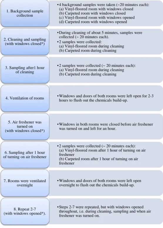
Chapter 3 Indoor air analysis: Analysis of VOCs in new buildings during and after cleaning and use of fragrance products 72 3.1 Introduction ... 73
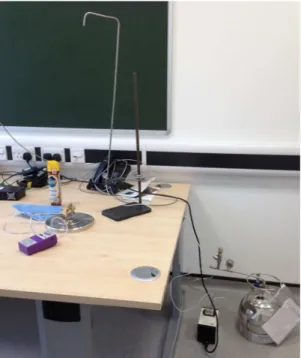
3.2 Test sites and conditions... 74
3.3 Thermal Desorption and GC instrumentation ... 77
3.4 Results and Discussion ... 78
3.5 Conclusion ... 86
Chapter 4 Sampling and analysis of cyclic volatile methyl siloxanes in air 87 4.1 Introduction to Cyclic Volatile Methyl Siloxanes ... 88
4.2 Internship in ACES, Stockholm University ... 93
4.3 Materials ... 94
4.4 Instrumentation ... 95
viii
4.6 Active sampling ... 109
4.7 Passive sampling ... 111
4.7.1 Passive sampling with sorbents in cartridges ... 111
4.7.2 Passive sampling using sorbents packed in bags ... 112
4.7.3 Cleaning of passive sampling bags ... 114
4.7.4 Positioning of sampling bags ... 114
4.7.5 Exploring different packaging of passive samplers ... 116
4.8 Calibration of passive sampling method ... 122
4.9 Storage of passive samplers in glass vials ... 127
4.10 Blank levels and LOD values ... 129
4.11 Real indoor air sampling in homes ... 130
4.11.1 Calibration ... 130
4.11.2 Results from real indoor air analysis of cVMS ... 131
4.12 Conclusion ... 141
Chapter 5 Development of a portable sensor device: Heating and detection 142 5.1 Introduction ... 143
5.2 Heating and cooling of the GC column ... 144
5.2.1 Temperature control of the Peltier device ... 146
5.2.2 Summary of using Peltier device as a temperature control ... 149
5.3 Separation performance of a laboratory GC-PID ... 149
5.3.1 Data capture with 12-bit ADC LabJack ... 153
ix
5.3.3 Summary of using PID as the detector method ... 160
Chapter 6 Development of a portable sensor device: Columns and separations 161 6.1 Preliminary LOC design ... 162
6.1.1 First set of PDMS LOC ... 163
6.2 Copper enclosure to contain GC column ... 166
6.3 Injection of gaseous sample into GC column ... 168
6.4 Detection of gaseous samples with PID ... 169
6.5 Future work... 179
6.5.1 GC LOC ... 179
6.5.2 Adsorption-desorption step prior to separation ... 180
6.5.3 Integration of parts that make up the sensor ... 181
Appendix A Chromatograms and mass spectra for indoor air analysis 183 Appendix B Consent form and Information Sheet for cVMS analysis in
homes 206
Appendix C Block diagram with code for Peltier device temperature
control 210
I
List of Figures
Figure 1-1. Ozone formation in the troposphere. ... 3 Figure 1-2. (a) Reaction of unsaturated compounds with ozone and (b)
formation of OH radicals from Criegee biradicals. ... 13 Figure 1-3. Structures of cVMS. From left – right: D3, D4, D5, D6. ... 14
Figure 1-4. Left: Packed GC column; Right: Capillary GC column. ... 17 Figure 1-5. Schematic of a typical laboratory set-up for the analysis of
gaseous samples. ... 22 Figure 1-6. Configuration of a sequential injection analyser where H =
hold-up conduit, FC = flow cell, R = reactor coil and AR = auxiliary reactor. ... 24 Figure 1-7. Micro sequential injection system (LOV) with the central
sample processing unit integrated with a flow cell for optical detection mounted atop a six-position valve. ... 25 Figure 1-8. Schematic of a paper-based electrochemical device, comprising
of a paper channel in conformal contact with the electrodes printed on a piece of paper. ... 26 Figure 1-9. Micro-reactor for the derivatisation of carbonyls. ... 28 Figure 1-10. (a) Layout of components in the temperature controlled stack
used for heating and cooling of the glass GC. (b) Plan view layout of the temperature controlled stack. ... 29 Figure 2-1. Work flow for sampling and analysis of samples from homes. ... 33 Figure 2-2. Schematics depicting (a) the flow path of gas during sampling
and (b) focusing trap desorption. ... 37 Figure 2-3. Diagram of a quadrupole mass analyser. ... 38 Figure 2-4. Diagram of a TOF mass analyser. ... 40
II
Figure 2-5. Extracted ion chromatographs of selected VOCs at the exact masses of their most abundant ion for one of the homes in London. ... 44 Figure 2-6. Mass spectra of isoprene (a) from Home 03 and (b) from NIST
MS library. ... 45 Figure 2-7. Mass spectra of toluene (a) from Home 03 and (b) from NIST
MS library. ... 46 Figure 2-8. Mass spectra of o-xylene (a) from Home 03 and (b) from NIST
MS library. ... 47 Figure 2-9. Mass spectra of α-pinene (a) from Home 03 and (b) from NIST
MS library. ... 48 Figure 2-10. Mass spectra of d-limonene (a) from Home 03 and (b) from
NIST MS library. ... 49 Figure 2-11. Mass spectra of tetrachloroethylene (a) from Home 03 and (b)
from NIST MS library. ... 50 Figure 2-12. Mass spectra of D5 (a) from Home 03 and (b) from NIST MS
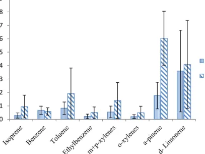
library. ... 51 Figure 2-13. Averaged concentrations of the most abundant indoor VOCs
from 19 homes in London showing the median, interquartile range, and the maximum and minimum values. ... 58 Figure 2-14. Comparison between homes with single-glazed windows and
double-glazed windows. ... 61 Figure 2-15. Reaction of limonene and OH. ... 63 Figure 2-16. Reaction of limonene and ozone. ... 64 Figure 2-17. Averaged concentrations of the most abundant indoor VOCs
from six similar build homes in York showing the median, interquartile range, and the maximum and minimum values. ... 65
III
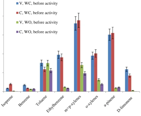
Figure 2-18. Variability in selected indoor VOCs of each of the homes in York, showing the median and the maximum and minimum values. ... 66 Figure 3-1. Work flow diagram of sampling carried out in new building. ... 75 Figure 3-2. Canisters attached with pump for active sampling of indoor air. .... 76 Figure 3-3. (a) Cleaning product and (b) fragrance used. ... 76 Figure 3-4. Concentrations of compounds before any activities were carried
out. (V = vinyl-floored; C = carpeted; WC = windows closed; WO = windows opened) ... 79 Figure 3-5. Concentrations of compounds detected across different
scenarios in rooms with vinyl and carpet flooring when windows were closed. (V = vinyl-floored; C = carpeted; WC = windows closed; WO = windows opened) ... 80 Figure 3-6. Concentrations of compounds detected across different
scenarios in rooms with vinyl and carpet flooring when windows were opened. (V = vinyl-floored; C = carpeted; WC = windows closed; WO = windows opened) ... 81 Figure 3-7. Concentrations of compounds in vinyl-floored room with
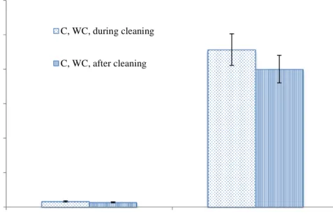
windows closed during and after cleaning. (V = vinyl-floored; WC = windows closed) ... 82 Figure 3-8. Concentrations of compounds in carpeted room with windows
closed during and after cleaning. (C = carpeted; WC = windows closed) ... 83 Figure 3-9. Concentrations of compounds in vinyl-floored room with
windows opened during and after cleaning. (V = vinyl-floored; WO = windows opened) ... 84
IV
Figure 3-10. Concentrations of compounds in carpeted room with windows opened during and after cleaning. (C = carpeted; WO = windows
opened) ... 84
Figure 3-11. Concentrations of compounds in vinyl-floored room with windows closed and opened after application of air fragrance. (V = vinyl-floored; WC = windows closed; WO = windows opened) ... 85
Figure 3-12. Concentrations of compounds in carpeted room with windows closed and opened after application of air fragrance. (C = carpeted; WC = windows closed; WO = windows opened) ... 86
Figure 4-1. ENV+ polymer. ... 92
Figure 4-2. ABN polymer. ... 92
Figure 4-3. Structure of M4Q. ... 94
Figure 4-4. Extracted ion chromatographs of D3, D4, D5, D6 and M4Q for the analyses carried out in Stockholm. ... 97
Figure 4-5. Extracted ion chromatographs of D3, D4, D5, D6 and M4Q for the analyses carried out in York. ... 98
Figure 4-6. Extracted ion chromatographs of D3, D4, D5, D6 and M4Q at exact masses for the analyses carried out in York. ... 99
Figure 4-7. Mass spectra of D3 (a) from 40 ppb standard and (b) from NIST MS library. ... 101
Figure 4-8. Mass spectra of D4 (a) from 40 ppb standard and (b) from NIST MS library. ... 102
Figure 4-9. Mass spectra of D5 (a) from 40 ppb standard and (b) from NIST MS library. ... 103
Figure 4-10. Mass spectra of D6 (a) from 40 ppb standard and (b) from NIST MS library. ... 104
V
Figure 4-11. Mass spectra of M4Q (a) from 40 ppb standard and (b) from NIST MS library. ... 105 Figure 4-12. Cartridges and frits from Biotage. ... 106 Figure 4-13. (a) ENV+ sorbent washed by hexane. (b) ENV+ sorbent dried
with filtered N2. ... 107
Figure 4-14. (a) & (b) Weighing of ENV+ sorbent into cartridges. (c) Top frit placed into cartridge, to be pushed in with a glass pipette. ... 108 Figure 4-15. A ready 1 mL cartridge filled with 10 – 15 mg of ENV+ sorbent. 108 Figure 4-16. (a) Wet ABN added directly into 1 mL cartridges. (b) ABN
dried with filtered N2. ... 109
Figure 4-17. Ratios of the relative areas of the compounds to their respective blanks for active sampling using ABN and ENV+ sorbents. ... 110 Figure 4-18. Ratios of the relative areas of the compounds to their respective
blanks for passive sampling using exposed ABN and ENV+ sorbents. ... 112 Figure 4-19. Ratios of the relative areas of the compounds to their respective
blanks for ENV+ sorbents in passive sampling bags. ... 113 Figure 4-20. Comparison of cVMS levels in passive sampling bags before
and after cleaning. ... 114 Figure 4-21. Ratios of the relative areas of the compounds to their respective
blanks for passive sampling bags placed in still and drafty locations. ... 115 Figure 4-22. (a) Nylon bags with 30 mg ENV+ sorbent prepared. (b) Slimmer
bags with 30 mg ENV+ sorbent. (c) Even thinner bags with 20 mg ENV+ sorbent... 116 Figure 4-23. Ratios of the relative areas of the compounds to their respective
VI
Figure 4-24. (a) Non-compartmentalised sampling bags design. (b) Compartmentalised passive sampling bags design to spread out
sorbents in bag. ... 118
Figure 4-25. Ratios of the relative areas of the compounds to their respective blanks for non-compartmentalised and compartmentalised passive sampling bags. ... 119
Figure 4-26. (a) Compartmentalised passive sampling bags design. (b) More compartmentalised passive sampling bags design. ... 120
Figure 4-27. Bags with different number of compartments, both containing 30 mg of ENV+ sorbent each. ... 120
Figure 4-28. Ratios of the relative areas of the compounds to their respective blanks for passive sampling bags with big and small compartments. ... 121
Figure 4-29. Passive sampling model. ... 122
Figure 4-30. (a) Blanks for passive sampling. (b) Passive samplers hung on a paper clip. ... 124
Figure 4-31. (a) Capped cartridge as blank for active sampling. (b) Two cartridges attached to pumps in parallel for active sampling... 124
Figure 4-32. Active sampling set-up with pumps and volumetric flow meter. .. 125
Figure 4-33. Analyte cVMS collected as a function of passive sampler deployment time. ... 126
Figure 4-34. (a) Vial with passive sampler attached to the cap with a string and tape. (b) Closed vial during storage and/or transport. (c) Passive samplers attached to the cap of the vial. Vial cap has an adhesive so it can be stuck onto any surface for sampling. ... 127
Figure 4-35. Percentage recovery of cVMS over the storage period. ... 128
Figure 4-36. Passive sampling bag in a sealed vial. ... 130
VII
Figure 4-38. Box and whiskers diagram showing the median and interquartile range of the concentration of cVMS in samples of homes
analysed. ... 135
Figure 5-1. Schematic diagram for sensor development. ... 144
Figure 5-2. Peltier device. ... 145
Figure 5-3. A Peltier device with a heatsink and a fan. ... 146
Figure 5-4. One temperature cycle of the Peltier device. ... 147
Figure 5-5. Five cycles of the Peltier device used for GC chip temperature control. ... 148
Figure 5-6. White container housing Peltier device and components ... 149
Figure 5-7. PID-AH purchased from Alphasense, placed next to a 20 pence for size comparison. ... 150
Figure 5-8. PID diagram. ... 151
Figure 5-9. Capillary column connected to a PID. ... 151
Figure 5-10. GC-PID set-up. ... 152
Figure 5-11. Separation of the 4 ppb standard gas mixture and detection by TOF/MS. ... 153
Figure 5-12. Separation of the 4 ppb standard gas mixture and detection by PID. ... 154
Figure 5-13. Separation of the isoprene and toluene gas mixture and detection by TOF/MS. ... 155
Figure 5-14. Separation of the isoprene and toluene gas mixture and detection by PID. ... 155
Figure 5-15. Separation of the 4 ppb standard gas mixture and detection by TOF/MS. ... 156
Figure 5-16. Separation of the 4 ppb standard gas mixture and detection by PID with 18-bit ADC... 157
VIII
Figure 5-17. Separation of the 4 ppb standard gas mixture and detection by
PID. ... 158
Figure 6-1. Preliminary design of GC – LOC on square-shaped chip. ... 162
Figure 6-2. (a) Side view of PDMS chip. (b) Top view of PDMS chip. ... 163
Figure 6-3. 5x magnification of PDMS chip. ... 163
Figure 6-4. (a) 20x magnification showing good consistency in the channels. (b) 20x magnification showing minor fabrication defects. ... 164
Figure 6-5. PDMS chip with needles fixed to the inlet and outlet of channels. ... 165
Figure 6-6. PDMS chip with PEEK tubing extensions at the inlet and outlet. . 165
Figure 6-7. (a) Copper enclosure with column. (b) Copper enclosure, containing column, covered with lid. ... 166
Figure 6-8. (a) Arrangement of the Peltier stack. (b) Peltier stack in a 3D printed block. ... 167
Figure 6-9. Sample injection for a two-position valve. ... 168
Figure 6-10. Set up of Peltier stack with a two-position valve. ... 168
Figure 6-11. (a) Headspace of standards were drawn up by a syringe. (b) Schematic set-up for headspace injection of standards into GC column. ... 169
Figure 6-12. PID chromatograph of isoprene and toluene mixture from GC separation with Peltier device. Carrier gas: N2. ... 170
Figure 6-13. PID chromatograph of mixture containing isoprene, toluene and ethylbenzene from GC separation with Peltier device.Carrier gas: N2. ... 171
Figure 6-14. Van Deemter plot for nitrogen, helium and hydrogen. ... 172
Figure 6-15. PID chromatograph of mixture containing isoprene, toluene and ethylbenzene from GC separation with Peltier device. Carrier gas: He. ... 173
IX
Figure 6-16. PID chromatograph of mixture containing isoprene, toluene and ethylbenzene from GC separation with Peltier device and heated transfer lines. Carrier gas: He. ... 174 Figure 6-17. PID chromatograph of mixture containing isoprene, toluene,
ethylbenzene and o-xylene from GC separation with Peltier device and heated transfer lines. Carrier gas: He. ... 175 Figure 6-18. PID chromatograph of mixture containing isoprene, toluene,
ethylbenzene and o-xylene from GC separation with Peltier device at isothermal temperatures and heated transfer lines. Carrier gas: He. ... 177 Figure 6-19. Schematic of a conducting-ink coated PLOT column for
X
Figure A-1. Analysis of Home 01: Detection by laboratory standard TOF/MS detector (a) from 2.5 – 8 min and (b) 8 – 12.5 min and (c) detection by PID. ... 184 Figure A-2. Analysis of Home 02: Detection by laboratory standard
TOF/MS detector (a) from 2.5 – 8 min and (b) 8 – 12.5 min and (c) detection by PID. ... 185 Figure A-3. Analysis of Home 03: Detection by laboratory standard
TOF/MS detector (a) from 2.5 – 8 min and (b) 8 – 12.5 min and (c) detection by PID. ... 186 Figure A-4. Analysis of Home 04: Detection by laboratory standard
TOF/MS detector (a) from 2.5 – 8 min and (b) 8 – 12.5 min and (c) detection by PID. ... 187 Figure A-5. Analysis of Home 05: Detection by laboratory standard
TOF/MS detector (a) from 2.5 – 8.5 min and (b) 8.5 – 16 min and (c) detection by PID. ... 188 Figure A-6. Analysis of Home 06: Detection by laboratory standard
TOF/MS detector (a) from 2.5 – 8.5 min and (b) 8.5 – 16 min and (c) detection by PID. ... 189 Figure A-7 Analysis of Home 07: Detection by laboratory standard
TOF/MS detector (a) from 2.5 – 8.5 min and (b) 8.5 – 16 min and (c) detection by PID. ... 190 Figure A-8. Analysis of Home 08: Detection by laboratory standard
TOF/MS detector (a) from 2.5 – 8.5 min and (b) 8.5 – 16 min and (c) detection by PID. ... 191 Figure A-9. Analysis of Home 09: Detection by laboratory standard
TOF/MS detector (a) from 2.5 – 8.5 min and (b) 8.5 – 12.5 min and (c) detection by PID. ... 192
XI
Figure A-10. Analysis of Home 10: Detection by laboratory standard TOF/MS detector (a) from 2.5 – 8.5 min and (b) 8.5 – 12.5 min and (c) detection by PID. ... 193 Figure A-11. Analysis of Home 11: Detection by laboratory standard
TOF/MS detector (a) from 2.5 – 8.5 min and (b) 8.5 – 12.5 min and (c) detection by PID. ... 194 Figure A-12. Analysis of Home 12: Detection by laboratory standard
TOF/MS detector (a) from 2.5 – 8.5 min and (b) 8.5 – 12.5 min and (c) detection by PID. ... 195 Figure A-13. Analysis of Home 13: Detection by laboratory standard
TOF/MS detector (a) from 2.5 – 8.5 min and (b) 8.5 – 13 min. .... 196 Figure A-14. Analysis of Home 14: Detection by laboratory standard
TOF/MS detector (a) from 2.5 – 8.5 min and (b) 8.5 – 13 min. .... 197 Figure A-15. Analysis of Home 15: Detection by laboratory standard
TOF/MS detector (a) from 2.5 – 8.5 min and (b) 8.5 – 13 min. .... 198 Figure A-16. Analysis of Home 16: Detection by laboratory standard
TOF/MS detector (a) from 2.5 – 8.5 min and (b) 8.5 – 13 min. .... 199 Figure A-17. Analysis of Home 17: Detection by laboratory standard
TOF/MS detector (a) from 2.5 – 8 min and (b) 8 – 14 min. ... 200 Figure A-18. Analysis of Home 18: Detection by laboratory standard
TOF/MS detector (a) from 2.5 – 8 min and (b) 8 – 14 min. ... 201 Figure A-19. Analysis of Home 19: Detection by laboratory standard
TOF/MS detector (a) from 2.5 – 8 min and (b) 8 – 14 min. ... 202 Figure A-20. Mass spectra of benzene (a) from Home 03 and (b) from NIST
MS library. ... 203 Figure A-21. Mass spectra of ethylbenzene (a) from Home 03 and (b) from
XII
Figure A-22. Mass spectra of m+p-xylenes (a) from Home 03 and (b) from NIST MS library. ... 205 Figure B-1. Sampling bag in vial. ... 209 Figure C-1. Block diagram with code for Peltier device temperature control. . 210
XIII
List of Tables
Table 1.1. List of indoor pollutants and their sources. ... 6 Table 1.2. List of commonly detected indoor VOCs and their possible
sources... 8 Table 1.3. Previous measurements of VOCs in homes ... 11 Table 1.4. Current measurement methods for VOCs. ... 18 Table 2.1. The detected compounds. ... 43 Table 2.2. List of compounds and their base peaks in a TOF mass spectrum. .... 52 Table 2.3. Characteristics of sampled homes in London. ... 54 Table 2.4. Ratios of concentrations of VOCs / benzene. ... 59 Table 2.5. Ratio of outdoor concentrations of VOCs / benzene. ... 59 Table 2.6. Activity log for York homes. ... 67 Table 2.7. Ratios of concentrations of VOCs / benzene. ... 68 Table 3.1. List of samples collected in new building. ... 77 Table 4.1. Information on cyclic volatile methyl siloxanes. ... 89 Table 4.2. Exact mass extracted ion analysis of cVMS and internal standard
M4Q with TOF/MS. ... 100 Table 4.3. LOD values of passive sampler. ... 129 Table 4.4. Concentrations of D3, D4, D5 and D6 in York homes. ... 133
Table 4.5. LOD values for cVMS analysis. ... 134 Table 4.6. Mininum, maximum and average concentrations of cVMS in
homes. ... 134 Table 4.7. List of cVMS concentrations at various locations with different
sampling and analysis methods. ... 139 Table 5.1. LOD of compounds with PID as detection method. ... 159
XIV
List of abbreviations
cVMS Cyclic Volatile Methyl Siloxanes D3 Hexamethylcyclotrisiloxane
D4 Octamethylcyclotetrasiloxane
D5 Decamethylcyclopentasiloxane
D6 Dodecamethylcyclohexasiloxane
DCM Dichloromethane
ENV+ Hydroxylated polystyrene-divinylbenzene copolymer GC Gas Chromatography
LOC Lab-on-a-chip
M4Q Tetrakis(trimethylsiloxy)silane MS Mass Spectrometry
PID Photoionisation Detector TD Thermal Desorption
TOF/MS Time-of-flight Mass Spectrometry VOC Volatile Organic Compounds
1
Chapter 1
Chapter 1 Volatile organic compounds
2
1.1
Volatile organic compounds
Volatile organic compounds (VOCs) are organic compounds with boiling points of less than or equal to 250 °C measured at a standard atmospheric pressure of 101.3 kPa 1. These compounds can have both direct and indirect impacts on
human health; VOCs contribute to the formation of photochemical smog and ground level ozone 2-4 and some VOCs, e.g. benzene and formaldehyde, are
considered to be carcinogens 2, 5-7. VOCs are emitted from natural and
anthropogenic (man-made) sources. Some natural sources of VOCs include vegetation, forest fires, and animals and these dominate the global budget of emissions 8. Although on a global scale VOC emissions are largely from natural
sources, air quality problems in populated and industrialized areas are mainly a result of anthropogenic sources 9. Some examples of anthropogenic VOCs include
tobacco smoke, biomass burning from human activities i.e. to exploit land for agricultural activities or to rid of agricultural waste, the production, storage and use of fossil fuels, and the production and use of household chemicals such as cleaning agents, coatings and paints.
In the troposphere, ozone formation occurs when ozone precursors react in the presence of sunlight (see Figure 1-1). The ozone precursors are nitrogen oxides and VOCs. VOCs contribute to the production of ozone, a constituent of photochemical smog that causes adverse health problems and also, when degraded in air, to the formation of organic aerosols. Ozone is formed in the atmosphere via a photochemical process whereby VOCs react with hydroxyl radicals in the presence of sunlight forming short-lived peroxy radical species (RO2). RO2 can
then react further rapidly converting NO to NO2, perturbing the natural
photostationary state. Photolysis of the NO2 formed then induces additional ozone
formation. Ground level ozone is a secondary pollutant and a harmful photochemical oxidant which inhabits that troposphere, and is the main
Chapter 1 Volatile organic compounds
3
component of photochemical smog 10. Photolysis of ozone occurs with the
absorption of solar ultraviolet radiation of wavelength shorter than 320 nm, resulting in excited O (1D) atoms which have sufficient energy to react with water
vapour to produce hydroxyl radicals.
VOC + OH → RO2 + H2O (Rate determining step) (1)
RO2 + NO → Secondary VOC + HO2 + NO2 (2) HO2 + NO → OH + NO2 (3) NO2 + hv (λ < 420 nm) → NO + O (Ground state) (4) O + O2 → O3 (5) O3 + hv (λ < 320 nm) → O2 + O (1D) (Excited state) (6) O (1D) + H 2O → 2OH + O2 (7)
Figure 1-1. Ozone formation in the troposphere.
Ground level ozone is notably important when it comes to public health. Ozone when inhaled can cause serious health problems such as breathing difficulty, inflammation of airways, declination of respiratory and pulmonary function and aggravation of lung diseases 11, 12. Exposure to ozone has also been associated
with respiratory morbidity and mortality 13-16, some populations, i.e. the elderly
and people with chronic conditions, being putatively more susceptible to ozone exposure 17, 18.
Ozone can be produced from simple hydrocarbons such as ethane, propane or from oxygenated compounds like formaldehyde and acetaldehyde. In indoor microenvironments and urban air, formaldehyde mixing ratios can vary from 1 to 100 ppb, while in remote clean oceanic areas formaldehyde is generally in the
[O2]
Chapter 1 Volatile organic compounds
4
range 0.1 – 1.0 ppb 19. Ethane and propane originate substantially from
anthropogenic pollution sources and have relatively long lifetimes against photochemical destruction. Background tropospheric mixing ratios of ethane and propane are 0.3 – 2.5 ppbv and 0.01 – 1.0 ppbv respectively. In addition to the production of ozone, acetaldehyde is also a precursor to peroxyacetyl nitrate (PAN), a secondary pollutant found in photochemical smog. It is a lachrymator and causes eye irritation. It has been reported that mixing ratios of PAN in clean air are typically 2 – 100 pptv, whereas that of polluted air can be as high as 35 ppbv 20. Other anthropogenic sources of VOCs include fuel combustion,
emissions from motor vehicles and evaporation of solvents and fuels 4 such as
ethene, toluene and benzene 21, 22. There are also biogenic sources of VOCs such
as the emissions of isoprene and terpenes from plants 23, 24 that can also be
important in the formation of ozone. The rapid and sensitive measurements of VOCs in ambient and indoor environments are therefore of great utility to environmental toxicology and atmospheric chemistry.
Chapter 1 Indoor air quality
5
1.2
Indoor air quality
The quality of air in the indoor environment in which we live and work has been gaining more attention and awareness because of its importance to the health and well-being of occupants 25. People in Europe spend at least 90% of their time
indoors 26 making this on a time weighted basis the dominant environment for
exposure. Two thirds of time indoors is spent at home, rendering the home environment a key setting for potential human exposure to air pollution 27. The
quality of air in the indoor environment is dependent on different factors such as the quality of the outdoor air, the building’s design and location, air change rates, furniture within the building, and the behavioural habits of the occupants 28.
While an important source of indoor air pollution is the air from outdoors, it is noted that pollutants could be also generated from indoor sources. In addition to the natural sources (such as from animals, moulds, plants and flowers) of indoor air pollution, there is a large number of anthropogenic sources as well i.e. smoking of cigarettes, burning of candles, cooking and cleaning activities, emissions from building material and paints, and usage of personal care products
28. Table 1.1 shows a list of indoor sources of pollution and some key indoor
pollutants 28, 29.
The potential health impacts as a result of exposure to compounds such as those listed in Table 1.1 have been discussed previously 30, 31. For instance, exposure to
formaldehyde can cause sensory and airway irritation, asthma and cancer; house dust mites, fungi and bacteria may cause asthma and produce allergic reactions in some people; NO2 increases susceptibility to infection, and therefore is a potential
hazard of respiratory illness. VOCs generally cover a wide range of compounds, some of which are known to have harmful effects on human health i.e. benzene 6
Chapter 1 Indoor air quality
6
humans by the International Agency for Research on Cancer 5, 33. New complex
substances could also be formed from the reaction between VOCs and oxidising compounds such as ozone 28.
Table 1.1. List of indoor pollutants and their sources.
Indoor sources Pollutants
Natural
Plants/flowers Animals (pets) Moulds
Dust mites and insects
Pollen Biological allergens Biological allergens Biological allergens Anthropogenic Air fresheners
Personal care products Cleaning products
Furniture, glues, insulation, carpets, cushions
Heating and cooking appliances
Building and insulation material
Cigarette smoke
VOCs VOCs VOCs
Formaldehyde, VOCs, dust mites
Particulates, nitrogen oxides, carbon monoxide, polycyclic aromatic hydrocarbons (PAHs), VOCs, ozone Mineral dusts and fibres e.g. asbestos
Environmental tobacco smoke including particulates, benzene and carbon monoxide
Chapter 1 Indoor air quality
7
1.2.1
VOCs in the indoor environment
Indoor pollutants include volatile organic compounds (VOCs), some of which have both short and long-term adverse health effects and which are directly classified as toxic or carcinogenic 34-37. VOCs are ubiquitous in any built
environment but there is considerable variation in speciation and abundance. These variation of VOCs found in homes depend on many factors such as emissions, ventilation and the oxidative environment and these are evolving over time, reflecting changes in chemical use, behaviour and building design/materials. Sources of indoor VOCs include ingress of outdoor pollution from traffic and industry, outgassing from building materials, flooring, electronic equipment and furnishings, emissions from food, cooking, cleaning products, personal care products, and from people and pets 26, 38, 39. Concentrations and speciation of
VOCs in the indoor environment can also be influenced by seasonality, duration of occupancy, personal activities such as smoking and showering, and even the education levels of the occupants 40-42. A list of some of the commonly detected
Chapter 1 Indoor air quality
8
Table 1.2. List of commonly detected indoor VOCs and their possible sources.
VOCs Sources
Alkanes, alkenes Isoprene Hexane Cyclohexane
Plants, human breath
Adhesives, aerosols in perfumes, gasoline Paints, thinners, adhesives
Aromatics Benzene Toluene Ethylbenzene Xylenes 1,2,4-Trimethylbenzene Naphthalene Styrene
Cigarette smoke, stored fuels, car exhausts Paints, thinners, adhesives
Paints, varnishes, pesticides, adhesives Paint, varnishes, adhesives
Gasoline, car exhausts
Cigarette smoke, insecticides, car exhausts Adhesives, cigarette smoke, car exhausts Terpenes
α-Pinene d-Limonene
Fragranced consumer / cleaning products Fragranced consumer / cleaning products Carbonyls
Formaldehyde Acetaldehyde Acetone 2-Butanone
Building materials, furniture, wood products Building materials, laminate, varnishes, paints Cleaning products, nail polish remover
Paint, adhesives, cleaning products, car exhausts Halogenated
Dichloromethane Tetrachloroethylene
Paint strippers, insecticides, hairspray, cleaners Dry-cleaned clothing
Chapter 1 Indoor air quality
9
Compared to half a century ago, there have been significant changes in the use of consumer products and building materials with impacts on both the concentrations and diversity of VOCs found indoors. In parallel there has been a move towards energy-efficient buildings with improved insulation and reduced air leakage and ventilation 43, 44. Sick or Tight Building Syndrome is a term that has been used to
describe circumstances whereby occupants within a building experience health-related effects or discomfort that seem to be health-related to the duration spent in a building. In such cases no specific cause can be found and relief from the symptoms, i.e. eye, nose and throat irritation and headaches, is typically experienced upon exiting or moving away from the building 45-48. These building
related symptoms have been reported to have increased discomfort and negative health effects, and result in reduced productivity at work and in schools 45, 49.
Many VOCs compounds can be oxidised to form more harmful secondary products, particularly if they contain reactive carbon double bonds 50-52. There
have been studies associating VOCs to negative health effects in humans; Billionnet et al. found that high concentrations of VOCs were associated with a higher risk of asthma and rhinitis in adults 53; Arif et al. reported that exposure to
VOCs may lead to adverse health consequences 54; Rumchev et al. reported the
association of VOCs with asthma in children 55, 56; results from the study by
Norbäck et al. suggested that indoor VOCs may be related to asthmatic symptoms
57.
Monoterpenes are one class of VOCs found indoors that have high reactivity with hydroxyl (OH) radicals, ozone and nitrate (NO3) radicals. Many hundreds of
different structures are possible in nature and they are released from a very wide range of sources including cooking, foodstuffs, plants and multiple kinds of fragranced products. In practice only a small number of monoterpenes are found in high abundance reflecting the common use of certain individual chemicals
Chapter 1 Indoor air quality
10
(such as d-limonene and α-pinene) in multiple products. There have been previous measurements of VOCs in homes (see Table 1.3) whereby high concentrations of particularly aromatics and terpenes were reported 39, 58-63.
Chapter 1 Indoor air quality
11
Table 1.3. Previous measurements of VOCs in homes
Study Location VOCs with highest concentrations Highest concentrations of VOCs (µg m-3) Reference
Chin et al. Homes in Detroit, Michigan, USA
Aromatics, terpenes (d-limonene and α-pinene), alkanes,
tetrachloroethene.
d-Limonene mean = 22.6
α-pinene mean = 4.4 Toluene mean = 11.62
39
Raw et al. Homes in England d-Limonene and toluene. d-Limonene mean = 6.2 Toluene mean = 15.1
58
Jia et al.
Homes in Ann Arbor, Ypsilanti and Dearborn in
Michigan, USA
Aromatics, chloroform, alkanes and terpenes.
d-Limonene mean = 25.7
α-pinene mean = 9.0 Toluene mean = 15.6
59
Villanueva et al. Homes in
Puertollano, Spain Alkanes, terpenes and aromatics.
d-Limonene mean = 17.1 α-pinene mean = 18.5 Toluene mean = 12.0 60 Schlink et al. Homes in Leipzig, München, and Köln, Germany
Aromatics, terpenes and alkanes.
Terpenes mean , median = 63.5, 36.1 Aromatics mean, median = 56.5, 37.2 Alkanes mean, median = 47.5, 24.0
61
Chapter 1 Indoor air quality
12 with d-limonene and α-pinene predominantly from indoor sources.
α-pinene mean = 11.5 Toluene mean = 15.5
Langer et al. Homes in Sweden Terpenes and toluene.
d-Limonene mean = 15.1
α-pinene median = 5.1 Toluene median = 7.3
Chapter 1 Indoor air quality
13
In terms of chemistry, d-limonene and α-pinene are unsaturated monoterpenes which are susceptible to ozonolysis by the electrophilic attack of ozone on the C=C double bonds, forming an unstable ozonide intermediate which breaks down into two possible combinations of a carbonyl and a Criegee biradical 64, 65.
Intermediate reactive radicals, such as OH, are formed in this reaction 64, 65 which
could further react with indoor VOCs and contribute to the further formation of indoor oxidised VOC products 66, 67. Oxidation products of d-limonene include
formaldehyde and 4-acetyl-1-methylcyclohexene, and those of α-pinene include formaldehyde, acetone and pinonaldehyde 68. Examples of the chemical reactions
are shown in Figure 1-2.
+
O3 R4 R3 R1 R2 O O O R1 R2 R4 R3 O R1 R2+
O C O R4 R3 O R3 R4+
C O O R2 R1 OzonideCriegee biradical Criegee biradical
O C O R4 R3 H H Criegee biradical O C O R4 C R3 H H O C R4 C R3 H
+
HOUnimolecular decay of Criegee intermediate to form OH radicals: (a)
(b)
Figure 1-2. (a) Reaction of unsaturated compounds with ozone and (b) formation of OH radicals from Criegee biradicals.
Chapter 1 Indoor air quality
14
1.2.2
Cyclic volatile methyl siloxanes in the indoor environment
Cyclic volatile methyl siloxanes (cVMS) are manufactured chemicals that are widely used in the production of personal care products and other consumer products such as fragrances, deodorants, lotions, toothpaste, household cleansers and furniture polishes 69-72. These cVMS include hexamethylcyclotrisiloxane (D3),
octamethylcyclotetrasiloxane (D4), decamethylcyclopentasiloxane (D5) and
dodecacyclohexasiloxane (D6) (D refers to the dimethylsiloxane unit, and the
subscript refers to the number of silicon bonds). As a result of their unique physiochemical properties of being inert and having a smooth texture, low surface tension, high thermal stability and good compatibility with other formulation ingredients, cVMS have become the basic ingredients as emollients or carrier solvents in the manufacture of consumer products. Figure 1-3 shows the structures of D3, D4, D5, D6. O Si O Si O Si Si O O Si Si O O Si O Si Si O Si O Si O Si O O Si O Si O Si O Si O Si O Si
Figure 1-3. Structures of cVMS. From left – right: D3, D4, D5, D6.
cVMS are of an environmental concern as they are potentially bioaccumulative and persistent with high octanol-water partition coefficient (log Kow) values > 5
and atmospheric oxidation half-life (AOt1/2) of more than 2 days 73. In addition to
these characteristics, cVMS are also highly volatile, and therefore have substantial potential for atmospheric long-range transport 74, 75.
There have been measurements of cVMS in the indoor and outdoor environments, with higher concentrations observed indoors 76-81. Previous studies have also
Chapter 1 Measurement of VOCs
15
reported high concentrations of cVMS in cosmetics and personal care products 69, 71; Wang et al. detected D
4, D5 and D6 concentrations as high as 11, 683 and 97.7
mg g-1 wet weight respectively in a sample of personal care products, cosmetics
and baby products in Canada 69; Horii et al. reported D
4, D5, and D6
concentrations of up to 9.38, 81.8 and 43.1 mg g-1 respectively in a sample of
cosmetics and personal care products obtained from retail stores in the USA and Japan 71. The high concentrations from cVMS in these products indicate that they
could be an important source of cVMS to the environment. In a recent study by Tang et al., cVMS, in particular D5, D4 and D6, contributed to about a third of the
total indoor VOC mass concentration indoor in a classroom, with their source largely associated to emissions from humans 82. cVMS were found to be the most
abundant VOC in a classroom with a distinct association with occupancy 83.
1.3
Measurement of VOCs
There is a range of different types of chemicals that are found in the indoor environment, and hence this necessitates the use of a complex method of analysis, such as gas chromatography - mass spectrometry, for the detection and quantification of the compounds found in indoor air samples.
There are numerous techniques and instruments used for the detection and measurement of VOCs, mostly based around gas chromatography (GC) and mass spectrometry (MS). Some examples are summarised in Table 1.4, together with the respective trade-offs of each method for field analysis. In very general terms, the development of a VOC instrument starts with laboratory standard devices, such as GC and MS, with modifications and additions then made to accommodate a trace level gaseous sample matrix. The key front-end adaptation to all chromatography-based systems is the inclusion of a thermal pre-concentration step, which strips VOCs from litre volumes of air and introduces them to the GC
Chapter 1 Measurement of VOCs
16
column with a concentration factor of up to 1000. A consequence is that most instruments in the literature for VOC detection are essentially hybrid lab instruments, not devices intrinsically designed with size, power or weight as constraining factors.
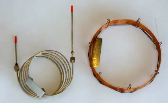
GC is a commonly used technique for the analysis of VOCs and it allows for the detection and quantification of a broad range of compounds that have reasonable volatility and thermal stability. There are two types of columns for GC: packed columns and open tubular columns (also known as capillary columns). Packed columns are generally made of glass or stainless steel, and are filled with the stationary phase or contain a solid support material coated with the liquid stationary phase. They are usually 1.5 – 6 m in length, and have diameters of 2 – 4 mm 84. Capillary columns, on the other hand, can have lengths as long as 100 m
and diameters as small as 0.1 mm, and therefore have higher efficiency (number of theoretical plates and separation power) 84. There are a few forms of capillary
columns: wall-coated open tubular (WCOT) columns, support-coated open tubular (SCOT) columns, and fused-silica wall-coated (FSWC) open tubular columns. In WCOT, the internal capillary wall is directly coated with a thin film of liquid stationary phase, whereas in SCOT the capillary wall is first lined with a thin layer of adsorbent solid, which is then coated with the liquid stationary phase. The FSWC column is a special type of WCOT that is drawn from pure silica and is much thinner than glass WCOT columns. The FSWC column is treated with a polyamide coating to protect it and allow it to be wound into coils. As a result of its flexibility, inertness and greater column efficiency, it is the most popular and commonly used column in analytical GC 84.
Figure 1-4 shows the two different types of GC column 85.
Given the limitations of current technologies for field analysis of VOCs, this work aims to address these issues and develop a portable sensor for the detection and
Chapter 1 Measurement of VOCs
17
analysis of VOCs, combining elements of thermal desorption (TD), gas chromatography (GC) and photoionsation detection (PID), but in a device built bottom up, rather than from standard lab equipment.
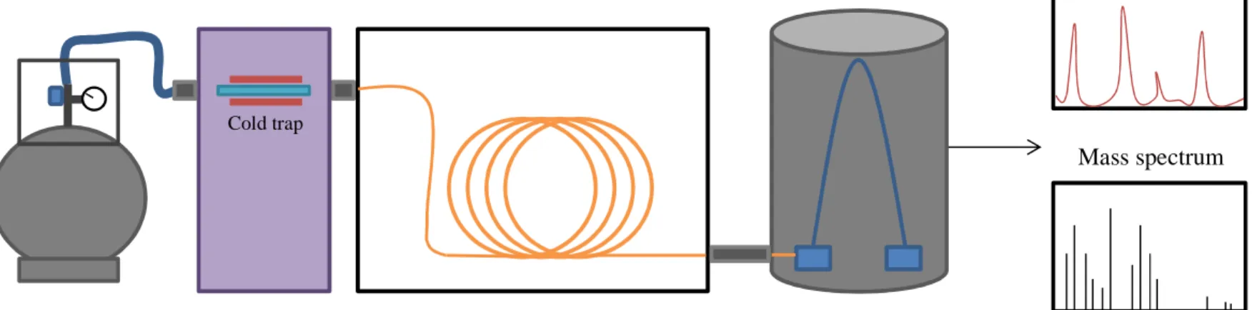
Figure 1-5 shows a schematic of a typical TD-GC-MS set up used in the laboratory for the analysis of gaseous samples (in silica-treated canisters).
Chapter 1 Measurement of VOCs
18
Table 1.4. Current measurement methods for VOCs.
Current measurement methods and its characteristics
Pros Cons
Thermal desorption - Gas Chromatography with Flame Ionisation Detectors (FID)
Most commonly used in laboratories for VOCs detection.
•Very sensitive and linear in response, and compound calibration can be based in part on a per carbon atom response function.
•Good in serviced laboratories or for fixed site observatories.
•Stable and reliable when operated autonomously.
•Not selective: The FID will respond to all organic compounds (except HCHO), so identification is based on retention times. Issues due to co-elutions; unable to identify unknown compounds.
•Not typically portable due to of its size, mass. Requirement for hydrogen gas is a major constraint on portability.
Bulk Photoionisation Detection (PID) Utilises an ultraviolet (UV) light source to break down VOCs in the air into positive and negative ions. Detection of the ions results in a current flow with a magnitude proportional to the concentration of
•Portable detector suitable for field applications because of its small size and no need for supply gases.
•The trade-off between using the PID or the FID in detection of VOCs has been discussed
86; the FID gave well-resolved peaks whereas
peak tailing was an issue when the PID was
•Operated in isolation the PID is not selective: will respond to all organic compounds.
•Each VOC has a different ionisation potential, which requires calibration.
Chapter 1 Measurement of VOCs
19
VOCs present. used. However, the low-power demands of the PID and its portability were advantages that the FID would not be able to provide.
Proton-Transfer-Reaction Mass Spectrometry (PTR-MS)
Air is pumped through a drift tube reactor, and a fraction of the VOCs is ionized in PTR with hydronium ions
87.
Soft ionization method; does not lead to fragmentation of the product ions. Reagent and product ions are measured by a quadrupole mass spectrometer; signal is proportional to the VOC mixing ratio.
•Allows numerous VOCs of atmospheric interest to be monitored with a high sensitivity (10 – 100 pptv) and rapid response time (1 – 10 sec).
•Does not require any sample treatment such as drying or pre-concentration, and is thus well suited for oxygenated VOCs, which cannot be quantified from canister samples.
•Provides a fast-response measurement of several key atmospheric VOCs, and complements the highly sensitive and chemically detailed snapshots obtained by GC techniques.
•Only determines the mass of product ions, which is not a unique indicator of the VOC identity.
•Isomers cannot be distinguished, and the interpretation of mass spectra is further complicated by the formation of cluster ions and the fragmentation of product ions.
•Not easily portable for field measurements.
Chapter 1 Measurement of VOCs
20 Thermal Desorption GC-MS
Sample collection using either packed adsorbent tubes of canisters. Samples preconcentrated by thermal desorption.
Typically uses quadrupole MS detection, but also increasingly TOF is applied.
•Sensitive and accurate means of retrospective analysis of VOCs adsorbed in soil samples 88, 89, other solids90, 91, liquids 92, 93 and gases 94-96.
•Sensitive and flexible, compound identifications available from mass spectra.
•Capable of identifying unknown compounds in an air sample via MS libraries.
•More sensitive from similar FID systems if operated in selected ion modes.
•Size and mass of the bench-top instrumentation render this method unsuitable for field analysis.
•More challenging to calibrate and less stable when operated continuously.
•Water can be a significant interference.
•Higher cost, more complex and typically requires thermostated lab environment for optimal operation.
•Several kilowatt power requirement.
Colorimetric (“Stain”) tubes i.e. Draeger tubes
Tube readings in the form of colour changes and intensities.
•Inexpensive method of measuring classes of toxic gases and vapours.
•Tubes have to be continuously observed to ensure that there is no sudden complete discoloration.
•Ultra-violet radiation may result in a change in the discoloration 97.
•Readings in the form of colour changes and intensities are subjected to human interpretation.
Chapter 1 Measurement of VOCs
21
•Not VOC specific. Metal Oxide Semiconductor (MOS)
sensors
•Compact and low cost sensors with high sensitivity and short response time.
•Also respond to inorganic gases 98: problem
when trying to measure trace or low concentrations of VOCs in the presence of gases such as NO, NO2 or CO which are found
in the surrounding air.
•Not favourable in the field measurement of VOCs because of the lack of selectivity and control of the sensor response.
Chapter 1 Measurement of VOCs
22
Figure 1-5. Schematic of a typical laboratory set-up for the analysis of gaseous samples.
Thermal desorption (TD) unit Gas chromatography (GC) Time-of-flight mass spectrometer (TOF/MS) Cold trap Silica-treated canister GC chromatogram Mass spectrum
Chapter 1 Miniaturisation through a lab-on-a-chip device
23
1.4
Miniaturisation through a lab-on-a-chip device
For the field measurement of VOCs, there is a need for a portable device that provides reliable information on a range of different VOCs, since the impact on downstream effects such as ozone and aerosol formation and health toxicology are structure-specific. Field measurements of VOCs are important in a range of disciplines including air pollution science, medical diagnostics and security screening. There is an enduring need for a portable device that provides reliable compound-specific measurements, at mixing ratios in the part per billion and part per trillion ranges. Bulk measurements (e.g. total carbon mass per unit volume) of VOCs do not provide sufficient detail on the precise VOC composition to be useful in most environmental and health applications. Any portable device should be robust, low-cost and have low-power demands, since many applications are likely to be off-grid. The development of a lab-on-a-chip (LOC) device requires a collaboration of multiple disciplines, involving research and development from different fields in sciences and engineering. This is necessary for the assembling and integration of sample collection and preparation stages, gas chromatography (GC) separation stage and photoionization detection (PID), to create a complete functional system.
The literature on GC-LOC dates back to 1970s: Terry et al. described the development of a miniaturised GC system whereby capillary channels and valves were fabricated on a silicon wafer by photolithography and chemical etching techniques, and a nickel resistor thermal conductivity detector was used as the detection method 99. The idea of miniaturization and LOC was a result of the
growing environmental demands for reduced consumption of sample and reagent solutions. There was a move towards the development of multi-analyte analysers that could be used for environmental monitoring purposes. The first generation of flow injection (FI) led to the development of the second generation sequential
Chapter 1 Miniaturisation through a lab-on-a-chip device
24
injection (SI) analysis in 1990 100 which was later followed by the creation of
lab-on-a-valve (LOV) in 2000 101. The LOV was seen as a downscaled analytical tool
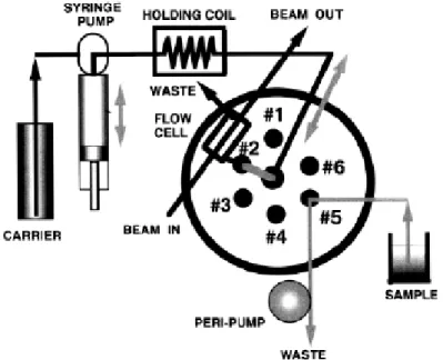
and fluidic universal system for reagent-based assays at the low microliter level, which was versatile and had the potential to incorporate different sample preparation procedures in its process. Figure 1-6 100 and Figure 1-7 101 show the
schematics of a SI analyser and a LOV respectively.
Figure 1-6. Configuration of a sequential injection analyser where H = hold-up conduit, FC = flow cell, R = reactor coil and AR = auxiliary reactor 100.
Chapter 1 Miniaturisation through a lab-on-a-chip device
25
Figure 1-7. Micro sequential injection system (LOV) with the central sample processing unit integrated with a flow cell for optical detection mounted atop a
six-position valve 101.
In the recent years, much intensive research has been conducted with regards to the miniaturizing of flow systems, resulting in the development of LOC (or micro total analysis systems, µTAS). The fabrication of such systems is to allow the automation of standard laboratory practices in a miniaturized format, with the obvious advantages of lower consumption of sample and reagents, possibility of separations with higher resolutions, low cost set-ups and shorter analysis duration
102. Another advantage pointed out in the same review paper by A Rios et al. is
that the automation of laboratory processes on a chip would reduce the need for highly skilled personnel to handle complex equipment 102. Much of the research
work on LOC has been predominantly carried out by electrical and mechanical engineers in research institutions. The channel network, which is made by various sophisticated procedures, such as micro-drilling, etching, photolithography, or laser erasing, is impressively exact and reproducible, allowing different channels
Chapter 1 Miniaturisation through a lab-on-a-chip device
26
profiles to be obtained. As mentioned by Miro and Hansen, these LOCs “can be made in inexpensive materials, namely silicon, glass, polymethyl methacrylate and polydimethylsiloxane, and mass-produced at low cost, in fact, at much lower expenditures than the LOV. However, the microfluidic devices are usually dedicated, that is, they have fixed architecture for predetermined chemistries.” 103
There is yet another interesting emerging technology that harbours similar aims and advantages brought about by LOC – to be affordable and robust, yet sensitive and specific for its usage. This emerging development is known as microfluidic paper-based analytical devices (µPADs) which comprises of microfluidic channels on paper instead of glass or plastic as in LOC devices. Movement of fluids within the channels in µPADs is via capillary action, hence eliminating the need for pumps or valving mechanisms to control fluid flow. Detection means for these devices are usually electrochemical or colorimetric 104-107. Figure 1-8 107
shows the schematic of a paper-based electrochemical sensing microfluidic device.
Figure 1-8. Schematic of a paper-based electrochemical device, comprising of a paper channel in conformal contact with the electrodes printed on a piece of paper. As a result of the portability of LOCs, its potential to be used for in-field real-time monitoring of the environment has been realised 108. There was the flexibility of
Chapter 1 Miniaturisation through a lab-on-a-chip device
27
resolution, and at low cost without the need to bring the samples back to the chemical laboratory for off-site analysis. Despite the obvious advantages brought about by LOCs, there are still doubts and criticisms on the real applicability of LOCs for real sample analysis. It has been said that “there is often no limitation as regards to the available volume of environmental sample as opposed to assays in the forensic, clinical and bioanalytical areas” 109, indicating that LOCs may be
redundant in the environment field. In the same review by Miro and Hansen, it was pointed out that the use of LOC with sample volumes of as low as nano-litre level may result in an issue with the representativeness of the sample obtained. It brings into question the reliability of the results when LOC is used as a mean of obtaining a measurement 109. In addition, LOC devices may not be developed
enough at this moment to cope with complex sample matrices, such as soil, which still requires sample preparation and clean-up procedures before they can be introduced to the LOC for detection. This is perhaps the biggest limitation faced by LOC devices in the environment field as they have to deal with the clogging of channels as a result of the introduction of particles that are present in the sample matrices.
1.4.1
LOC for gas phase analysis
Much of the problems and concerns associated with LOC are to do with the sample preparation of complex matrices, such as aqueous and soil samples from the environment that require clean-up steps prior to the detection of the desired analytes in these samples. There have been, however, reports of promising developments in the field of gas phase sensors involved in sample preparation procedures prior to detection and analysis of the analytes. A microfluidic lab-on-chip derivatisation technique has been optimized to achieve a rapid, automated and sensitive determination of ambient gaseous formaldehyde when used in combination with GC-MS. The method used a Pyrex micro-reactor comprising
Chapter 1 Miniaturisation through a lab-on-a-chip device
28
three inlets and one outlet, gas and fluid splitting and combining channels, mixing junctions, and a reaction micro-channel. The micro-reactor integrated three functions, that of: mixer and reactor, heater, and preconcentrator. The flow rates of the gas sample and derivatisation solution and the temperature of the micro-reactor were optimized to achieve a near real-time measurement with a rapid and high efficiency derivatisation step following gas sampling. The enhanced phase contact area-to-volume ratio and the high heat transfer rate in the micro-reactor resulted in a fast and high efficiency derivatisation reaction 19. This concept has
also proven to be successful for the derivatisation of other carbonyls, with method detection limits (MDLs) below or close to their typical concentrations in clean ambient air 110. Microfluidic derivatisation is attractive for many reasons; of
relevance here for field measurements are its economical consumption of reagents and energy. An advantage of undertaking reactions in microfluidic systems is that enhanced reaction efficiency may be achieved due to a high phase contact area-to-volume ratio in micro-channels.
Figure 1-9 shows the layout of the micro-reactor used for the derivatisation of the carbonyls 110.
Figure 1-9. Micro-reactor for the derivatisation of carbonyls.
One important factor for good GC separations is the uniform heating of a GC column. The heating of GC columns by conventional means is primarily based on the turbulent fan oven, which is an excellent means to achieve even heating of the column. However the size of such ovens renders this a difficult technique to use in