CAN MACHINE LEARNING IMPROVE
RECESSION PREDICTION ACCURACY?
Azhar Iqbal1, Kyle Bowman2
1Wells Fargo Securities, LLC, Charlotte
2Wells Fargo Bank, N.A., Charlotte
Abstract
This paper proposes a framework to utilize machine learning and statistical data mining tools in the economics/financial world with the goal of more accurately predicting recessions. Decision makers have a vital interest in predicting future recessions in order to enact appropriate policy. Therefore, to help decision makers, we raise the question: Does machine learning and statistical data mining improve recession prediction accuracy? Our first method examined over 500,000 variables as potential predictor variables for recession forecasting. Furthermore, to obtain the final logit/probit model specification, we ran 30 million different models. The selected model was then utilized to generate recession probabilities. The second method is the random forest approach, a famous class of machine learning tools. The third approach we employ is known as gradient boosting, a technique that also belongs in the machine learning family. Moreover, we built an econometric model that utilizes the yield curve as a recession predictor and employ that model as a benchmark. To test a model’s accuracy, we employ both in-sample and out-of-sample criteria. In our tests, the random forest approach outperforms all the other models (gradient boosting, statistical machine learning and the simple econometric model) in both the in-sample and out-of-sample situations. The gradient boosting model comes in second place, while the statistical data mining approach captures third. Furthermore, if we combine all four probabilities, then that method is still unable to beat the random forest’s prediction accuracy. That is, the random forest approach, alone, is the best. Our analysis proposes that machine learning can improve recession prediction accuracy. Moreover, our models suggest a less than 5% chance of a recession during the next 12 months.
Key Words: Recession Prediction; Machine Learning; Statistical Data Mining; Logit/Probit; Yield Curve.
INTRODUCTION
“Computers are useless. They can only give you answers.” Pablo Picasso
and statistical data mining tools in economics/financial world. The proposed framework employs to predict recessions. Decision makers have a vital interest to predict future recessions accurately as different set of decisions are needed for a recession than those of an expansion phase of a business cycle. Therefore, to help decision makers, we raise a question whether machine learning and statistical data mining improve recession prediction accuracy?
Our first method to predict recession is the statistical machine learning (also known statistical data mining). The estimation method is logit/probit modeling approach. This method utilized over 500,000 variables as potential predictors. Furthermore, to obtain the final logit/probit model specification, we ran 30 million different models. Then the selected model is utilized to generate recession probabilities.
The second method is the random forest approach which is a famous class of machine learning tools. The random forest approach utilizes the same set of predictors which are utilized in the statistical machine learning method. The third approach we utilize is known as the gradient boosting and it is also belong to the machine learning family. We also build an econometric model which utilizes the yield curve as a predictor and that model is employed as a benchmark. Basically, our benchmark model rely on an economic/financial theory as the yield curve is a famous recession predictor. Other three approaches include hundreds of thousands of potential predictors and those methods do not utilize any prior economic/financial theories. Therefore, we raise question whether the machine learning tools beat (provide more accurate forecast) a simple econometric model (a model with only one predictor)?
To test a model’s accuracy, we utilize both in-sample and out-of-sample criteria. The random forest (machine learning) approach outperform all other models which are the gradient boosting, the statistical machine learning and the simple econometric model in both the in-sample and out-of-sample criteria. The gradient boosting is at the second place and statistical machine learning capture the third position. Furthermore, if we combine all four probabilities then that method is unable to beat random forest’s prediction accuracy. That is, the random forest approach is still the best. Therefore, our analysis suggests that machine learning can improve recession prediction accuracy. Our models suggest a less than 5% chance of a recession during the next 18 months.
accuracy/reliable answer may not depends on computers (machine learning/big data) but how one utilize those computers.
PREDICTING RECESSION IN THE BIG DATA AGE: SETTING THE STAGE
Accurately predicting recessions is crucial for decision makers who are tasked with designing bespoke policy responses. Every recession is unique in the sense that different recessions have varying drivers. For example, one of the major causes of the Great Recession was the housing sector, while the IT boom/bust was a major cause of the 2001 recession. Knowing what will cause the next recession is a trillion dollar question. However, finding the right set of predictor variables to forecast the next recession is challenging because of the changing nature of the economy. Likewise, including too many variables in a traditional econometric modeling approach creates issues, such as an over-fitting problem (Please go to the end of the paper and see Note 1).
Machine learning tools, on the other hand, are capable of handling a very large set of variables while providing useful information to identify the target variable. Basically, in the machine learning approach, we are letting the data speak for themselves and predict recessions. The rationale is that recessions are the results of imbalances/shocks that must reveal themselves in certain sectors of the economy. By including information from various sectors of the economy, we can improve the prediction of those imbalances and corresponding recessions. One major challenge for today’s modelers is the abundance of information, where noise in large data sets can prove distracting. This challenge is different than the traditional modeling process where too little information was the issue. In the following sections we provide a reliable framework to utilize machine learning tools and large dataset (big data) to generate accurate recession forecasts.
Statistical Machine Learning: Opening Doors, Finding Connections
Our first recession prediction method is statistical machine learning, which is sometimes referred to as statistical data mining. In statistical machine learning modeling, we can “train” machines to go through hundreds of thousands of potential predictors and select a handful of predictors (4 to 6 variables, for example). That is, machines will utilize some statistical criteria (forecast error for instance) to narrow down the large dataset of potential predictors to a more manageable variable-list. We asked machines to consider over 500,000 variables as potential predictors and return to us a combination of five variables that predict U.S. recessions accurately.
practical to re-evaluate existing relationships and, if needed, add/subtract variables to/from a model. Statistical data mining does not rely on any economic/financial theory but identifies relevant variables using statistical tools. Second, complex economic interactions between different sectors vary over time as well. Thus the question, “what will cause the next recession?” is a very difficult one to answer. Therefore, putting everything in the pot (statistical data mining) increases the chances of finding what is affecting the target variable (recession) in the recent periods.
Third, it is important to note that a combination of some factors may bring about a recession rather than weakness in a single sector. For example, a drop in equity prices (S&P 500 index) and house prices along with a rising unemployment rate may be more likely to pull the economy into a recession than, for example, weakness in the manufacturing sector alone. Statistical data mining would likely help an analyst explore deep and complex interactions between different sectors that are closely associated with the target variables.
An added benefit of using statistical data mining is that important connections between different sectors are often unknown to analysts. Statistical machine learning can help an analyst identify those obscure connections. A great illustration of such unknown connections between certain sectors of the economy is the financial crisis and the Great Recession. That is, the housing boom was initially thought to be a regional phenomenon that would not pose a serious risk to the national economy. The Federal Open Market Committee (FOMC) transcripts from this period show that at first the FOMC considered there to be isolated regional housing bubbles. Likewise, by 2006, the meeting transcripts show that Ben Bernanke, the Federal Reserve Board’s Chairman at the time, discussed that falling home prices would not derail economic growth (Please go to the end of the paper and see Note 2). Furthermore, the relationship between the housing market and financial sector was
also underestimated and only appeared with the Lehman Brother’s bankruptcy in September 2008. Statistical machine learning has the potential to uncover such complex connections by utilizing information across major sectors of the economy.
Information Magic: How Does Statistical Machine Learning Work?
Here we outline our proposed framework to effectively utilize statistical machine learning to forecast recessions. It is important to note that here we are using recession prediction as a case study but our framework is flexible and would help an analyst to effectively utilize the statistical machine learning to obtain accurate forecasts for any variable of interest. The first step is to define the target variable (what we are forecasting?) which, in our case, is a recession. We utilize the National Bureau of Economic Research’s (NBER) definition of recession dates to construct the dependent variable. The dependent variable is a dummy variable with a value of zero (the U.S. economy is not in a recession) and one (the U.S. economy is in a recession). The benefit of using a dummy variable as the target variable is that we can generate the probability of a recession for a certain period-ahead using predictor variables.
Before we look for predictors, we need to discuss the sample period of the study. We started our analysis from January 1972 (monthly dataset). There are some major reasons to pick 1972 as a starting year of the analysis. First, since our dependent variable is a dummy variable that includes recession (value equals one) and non-recession (value equal zero) periods, our sample period must include both recession and non-recession periods. There have been six recessions since 1972. Second, many variables go back to the early 1970s and, therefore, provide an opportunity to select a model’s relevant predictors from a large dataset of potential predictors. As mentioned earlier, a large pool of potential predictors captures information from all major sectors of the economy, which provides an opportunity to detect obscure connections between different sectors, thereby improving forecast accuracy.
The final and most important reason for starting our analysis in 1972, is that it can provide enough observations in our modeling approaches to conduct both in-sample analysis and out-of-sample forecasting, helping us test the predictive power of all potential variables. That is, we utilize the 1972-1988 period for in-sample analysis and the 1989-2017 period is employed for of-sample forecasting purpose. What are in-sample analysis and out-of-sample forecasting? Why do we need to conduct in-sample and out-out-of-sample forecasting analysis?
out-of-sample process involves forecasting, and the model does not know (have information) about the actual outcome for the forecast-horizon at the time of forecasting. That is, we utilize the 1972-1988 period and ask the model to generate the probability of a recession during the next 12 months (forecast horizon is 12 months). The important point here is that the model does not know whether there is a recession during the next 12 months. Out-of-sample forecasting utilizes the available information to forecast a future period. Put simply, in- sample analysis utilizes the available information and provides a statistical relationship between the target variable and predictors for that sample period. Out-of-sample forecasting uses the discovered relationship between variables to predict the future values of the target variable (Please go to the end of the paper and see Note 3).
Now we turn to the next question of why we need to conduct in-sample and out-of-sample analyses. The in-out-of-sample analysis is a very effective tool to reduce the large potential list of predictors (sometimes the list contains hundreds of thousands or millions of potential predictors) to a more manageable pool. There are a number of statistical tests available within the in-sample analysis, which helps analysts identify a handful of predictors from the larger pool.
The out-of-sample forecasting exercise, in our view, is the most important tool in selecting the final model and improving forecast accuracy. When we generate the probability of a recession in real time, we will not know whether there will be a recession in the next 12 months. This is essentially a simulated real time forecasting experimentation. There are two major benefits of the simulated real time out-of-sample forecasting experiment. First, a common issue with forecasting models selected with using only in-sample selection criteria is over-fitting. Typically, an over-fitted model performs well during the in-sample analysis but very badly during out-of-sample forecasting. A model selected based on the out-of-sample forecasting criterion would reduce the over-fitting problem and improve forecast accuracy significantly compared to a model that is selected using in-sample criteria. The second major benefit is that the simulated real time out-of-sample forecasting would help an analyst estimate a reliable potential risk to the forecast (such as an average forecast error).
TURNING COLORS INTO A PICTURE: SAMPLE PERIOD AND DATA REDUCTION STEPS
(three recessions in the 1972-1988 period) and in the out-of-sample forecasting period (three recessions in the 1989-2017 period). The three recessions of the 1989-2017 period contain different characteristics (different depth and duration, for example) such as the 2007-2009 recession, which is the deepest recession since the Great Depression and hence has been labeled the Great Recession. The 2001 recession, on the other hand, is one of the mildest recessions in the sample era while the 1990-1991 recession is widely considered a moderate (neither mild nor deep) recession.
The major benefit of this out-of-sample forecasting simulation is that we do not know whether the next recession will be mild, moderate or deep; historically, mild recessions are relatively difficult to predict. If a model can predict recessions of different depths in a simulation, then there is a decent probability that the model would repeat its accuracy in the future.
A Sea of Potential Predictors: The FRED Dataset
One major benefit of the advancement of the Internet is that large datasets are available in a ready-to-use format, often at no cost. One such dataset is available on the Federal Reserve Bank of St. Louis’ website, commonly referred to as the FRED (Federal Reserve Economic Data) (Please go to the end of the paper and see Note 4).There are more than 500,000 variables
listed in FRED, collected from 86 different sources. For our analysis, we consider all the 500,000 variables as potential predictors and try to find reliable predictors from this dataset using statistical tools. As mentioned earlier, instead of picking a handful of predictors (a traditional modeling approach), we include everything in the pot to find useful predictors from over 500,000 variables (statistical data mining approach). By using all FRED data, one thing is certain, not all of the 500,000 variables are relevant to predicting recessions. Put differently, we are including lots of noises in the model in addition to useful signals. However, there are some major benefits, as discussed earlier, of using the entire FRED data. That is, we will be able to find some obscure/new connections between different sectors of the economy and those connections may improve recession prediction accuracy.
that may give an opportunity to analyze over 200,000 variables as potential predictors instead of under 6,000 variables in the present case. However, that analysis (1995 as starting year), will have a very serious issue and that issue would reduce recession prediction accuracy significantly. Why? There are only 2 recessions in the 1995-2017 period and that indicates we have to rely only on in-sample analysis and in-sample analysis is known for over-fitting problem. By the same token, 1990 as a starting years would add one more recession in the analysis (3 recessions in the 1990-2017 period) but again not enough observations/time span to conduct out-of-sample simulation. Once more, an analyst have to rely on in-sample analysis and potentially suffer with the over-fitting problem (Please go to the end of the paper and see Note 5).
The third and final point we want to stress is that we must employ an appropriate simulated real time out-of-sample analysis to finalize a model. Sometimes, as in the present case, an analyst may face a tradeoff between longer time span vs. a large pool of potential predictors. That is, if utilize longer time period (with starting year of 1972) then potential pool reduce from over 500,000 variables to 5889 variables. On the other hand, a 200,000 plus list of potential predictors is attached with a short time span (from 1995 and that period contains only 2 recessions). Our analysis picks a longer time span (over 200,000 potential predictors list) with a decent size of potential predictors (5889 variables as potential predictors). A shorter time span, let’s say 1995 as a starting year, will have only 2 recessions and that means our target variable will have lots of zeros (dummy variable with zero for no-recession and one for recession) and very few ones which naturally create a bias toward zeros. Therefore model will tend to predict very low probability of a recession and increases chances of a false negative scenarios (very high likelihood of missing a future recession).
information to find useful predictors and explore some possible connections between different sectors.
A Statistical Spell of Variables Reduction
The list of 5,889 potential predictors is large enough to conduct in-sample analysis and out-of-sample simulation. To obtain a more manageable set of predictors, we employ several statistical methods and utilize the complete sample period of 1972-2017. First, we run the Granger causality test between our target variable and each of the 5,889 variables
(Please go to the end of the paper and see Note 6). The Granger (1969) test is a precise method to find
which variables are statistically useful to predict the target variable (Please go to the end of the paper and see Note 7). For the Granger causality test, we set a 5% level of significance and keep
all variables that produce the p-value of the Chi-square test less than or equal to 0.05 (Please go to the end of the paper and see Note 8).
The next methods to reduce the number of variables is called Weight of Evidence (WoE) and Information Value (IV) (Please go to the end of the paper and see Note 9). Both the WoE and IV are
very good tools to find reliable predictors, particularly if dealing with a binary, dependent target variable (zero for no recession and one for recession). The WoE provides evidence of predictive power of a variable relative to the target variable. The IV method, on the other hand, helps to rank variables according to their predictive power (the Y-variable has a higher predictive power than the X-variable to forecast recession, for example).
The Granger causality test, WoE and IV methods help us reduce the list of 5,889 variables to a set of 1,563 potential predictors. However, 1,563 variables as potential predictors are a lot for the in-sample analysis and out-of-sample simulation. Therefore, we utilize economic theory and intuition to further narrow down the list of 1,563 variables. That is, we manually inspect these 1,563 variables and then categorize them to represent major sectors of the economy. For example, consider the category “current population survey.” A few potential predictors in this category are civilian labor for men only, White, Black, 16-19 year old and so forth. Not all of these series make economic sense to predict recessions, thus we remove them.
FINDING THE BEST SET OF PREDICTORS FOR RECESSION FORECASTING: DISCOVERING HIDDEN CONNECTIONS
We have now narrowed down the list of potential predictors to 192 variables. Next, we need to classify those 192 variables into categories. For example, we created the category “inflation” and put all inflation related variables (i.e. CPI and PCE deflator) in that category. Likewise, nonfarm payrolls and unemployment rate fall in the “employment” category and so on. We end up having 40 different categories. The 192 variables we have selected as potential predictors are individually statistically useful to predict recessions. Now we need to find the ideal combination of predictors that represent different sectors of the economy.
As we know, economies evolve over time and the strength of relations between different sectors of an economy also vary. Our approach will find a set of sectors that are statistically more accurate to predict recessions than any other set in our analysis. Basically, we utilize all possible combinations of the 192 variables and, by doing so, we explore the hidden connections between different sectors. Furthermore, including one variable from a category at a time avoids the potential multi-collinearity problem(Please go to the end of the paper and see Note 10).
We Ran 30 Million Regressions
Here is the outline of our procedure to find the best set of predictors from the 40 different categories. We set a logit/probit modeling framework with eight predictors (nine variables in a model: one dependent variable and eight predictor variables). Moreover, we are interested in a distinct combination of the eight predictors, meaning we want eight predictors from eight different sectors. For example, we pick the unemployment rate as a predictor from the “employment” category and the next predictor comes from the “inflation” category (CPI for example), the S&P500 from “equity”, 10-year Treasury yield from “interest rates” and housing starts from the “housing” category and so on. Therefore, eight predictors represent eight different sectors of the economy. In addition, we repeat the process by keeping the unemployment rate (to represent “employment”) in the model but change the rest of the predictors of the model one by one. That is, we include eight predictors at a time and then replace predictors with others, but keep the total number of predictors to eight. Why do we do this?
but also team up with other sectors to predict recessions. Therefore, we employ all possible combinations of these 40 categories and 192 variables and that process allows us to explore hidden connections between different sectors and improve recession prediction accuracy. The process is very time-intensive, taking several weeks of continuously running code. In total, we ran 30 million different models. We utilize the Schwarz information criterion (SIC) to narrow down 30 million models to a manageable list of models. We selected the top 1,500 models in this step using the SIC values (as we know a model with the lowest SIC value is the preferred one among competitors). The selected 1,500 models contain eight predictors in each model but all those models include distinct combinations of the eight predictors.
From the 1,500 different combinations of eight-predictors we need to select the final model (one model with eight predictors). Moreover, these 1,500 models were selected by using in-sample criterion, however, our objective is to forecast future recessions accurately (sample forecasting). Therefore, we utilize simulated real time out-of-sample forecast error as the criterion to find the best model among the 1,500 models.
Precisely, we utilize the 1972-1988 period to generate the probability of a recession during the next 12 months and then re-estimate the model using the 1972-1989: 1 period (include the next month in the estimation period) and again generate probability of a recession for the next 12 months. We iterated this process till we reached the last available data point, which is December 2016. The major benefit of this recursive forecasting is that we know the actual outcome (recession or no recession during the next 12 months), but we did not share that information with the model. This allows us to calculate the model’s accuracy. We repeat this process for each of the 1,500 models and select the model with the highest accuracy. That is, we select the set of eight-predictors, which forecast recessions during the 1989-2017 (period for the simulated out-of-sample forecasting) more accurately than the rest of the 1,499 models. Basically, we ran over half a million (504,000) simulations to select final model. The selected logit/probit model is utilized to represent the statistical machine learning/data mining approach.
HAPPY HUNGER GAMES: AND MAY THE ODDS BE EVER IN YOUR FAVOR
Who Perform the Best?
predictors are utilized to represent the data mining approach. The random forest and gradient boosting methods are utilized to represent machine learning.
Before we introduce a statistical tool to evaluate a model’s performance, we will discuss our precise objective about the target variable. That is, our target is to predict recessions accurately and our dependent variable is binary with zeros (non-recessionary periods) and ones (recessions). Furthermore, an accurate forecast from a model correctly predicts either a recession or a non-recessionary period in the forecast horizon. By the same token, an inaccurate forecast implies missing of a recession/non-recession. Precisely there are the following possibilities for a forecast:
(1) True positive: model correctly predicts recession;
(2) True negative: model accurately predicts non-recessionary period;
(3) False positive: model predicts a recession when there was no recession; and (4) False negative: model predicts non-recession but there was a recession.
With this information, we can restate our objective: a forecast should be true positive and true negative and avoid both false negative and false positive.
In addition, adjusting the probability threshold for a recession directly influences the changes of false positives. For example, 60% or higher probability indicates a recession, otherwise no recession. That threshold helps reduce chances of false positives. However, a higher probability-threshold also poses the risk of missing a recession. On the other hand, a threshold using a lower probability (20% probability as a threshold, for instance) would lead to more false positives. With this discussion in mind, we can introduce our statistical method to evaluate forecasts of a model.
The Relative Operating Characteristic (ROC) Curve
The relative operating characteristics (ROC) curve is a helpful tool to evaluate a model’s performance (Please go to the end of the paper and see Note 11). The ROC curve helps to find an optimal
threshold by plotting different thresholds’ performances. Put differently, the ROC curve shows a plot of a true positive (correct forecast) against a false positive (false signal) of a given threshold. Essentially, the ROC curve depicts accuracy (true positive vs. false positive) of different thresholds and the threshold which produces the highest accuracy can be selected. That is, a threshold can be identified by the ROC curve which produces the maximum hit rate along with least false signals.
value close to one represents higher accuracy while a value near zero represents a useless model. Therefore, the ROC AUC will help us determine which model is the best among competitors. Furthermore, we will estimate the ROC and ROC AUC for both in-sample analysis (complete sample period) and out-of-sample forecasting simulation (1989-2017) for each of the four models to evaluate which model is the most accurate.
The Legends of Machine Learning: The Random Forest and the Gradient Boosting Approaches
Applications of machine learning techniques in economics/finance are a relatively new phenomenon (Please go to the end of the paper and see Note 12). The basic logic behind machine learning
techniques is to utilize the available information effectively to generate accurate predictions. That is, machine learning techniques allow us to transform a computationally-hard problem into a computationally-efficient solution. In contrast to the traditional econometric techniques, which worry about issues such as linear/non-linear, small/large samples and degree of freedom/more predictors than observations etc., machine learning techniques find a connection between the target variable and predictors and then utilize that information to form a prediction. Put differently, most machine learning techniques divide data into segments and then utilize some of those segments for estimation and others for validation.
The basic idea behind most machine learning techniques is that an algorithm sets a loss function (minimum forecast error, for example) and finds a combination of predictors that produce a minimum forecast error, on average, among competitors. Before we discuss our models, we need to clarify one more thing, which is the classification and regression problem. In machine learning, if the target variable is binary (or categorical), then it is called a classification-problem while for a continuous-target variable the term regression-problem is utilized. Since our target variable is binary, we are dealing with a classification problem.
The Random Forest Approach
A tree, in simple words, successively chooses each predictor by splitting variables into two groups (partisans) and calculates the mean squared error (MSE). The tree splits at the point that minimizes MSE. The splitting process continues by further splitting each group into two new groups and calculates the MSE for each new group. Typically, in machine learning, these splitting points are called nodes. The splitting process continues until the stopping point is reached and the end point is labeled as leaves. A decision tree is simple to build and generates a very good in-sample fit but a horrible out-of-sample forecast. One major reason for bad out-of-sampling is that such trees are built using in-sample information and, typically, do not include out-of-sample forecasting.
Breiman (2001) improved the decision tree approach and his framework is known as the random forest (Please go to the end of the paper and see Note 13). The basic logic behind the random
forest approach is that instead of generating one tree, we can create many trees (number of trees can be in thousands or millions depending on the objective). Furthermore, if trees are independent and unbiased, then the average of those trees would be unbiased with a potentially small variance, and more likely to produce a better out-of-sample forecast. The averaging of different trees is called ensemble learning or the random forest approach. Essentially, averaging many models tends to provide better out-of-sample forecasts than a single model.
The Gradient Boosting Approach
The gradient boosting is also an ensemble approach and a very powerful machine learning tool for forecasting. The basic idea behind the gradient boosting is that a weak learner (in-accurate model) can be modified to become a better one (accurate model). A weak model can be defined as a model which produce a slightly better forecast than a random chance. Furthermore a tree (or decision tree) can be considered a weak learner as trees are infamous for very bad out-of-sample forecast. Friedman (1999) provides a formal framework to estimate a gradient boosting model (Please go to the end of the paper and see Note 14).
Essentially, in the gradient boosting modeling approach, we set a loss function (minimum MSE, for example) and then add weak learners (trees for example) to optimize the loss function using a gradient descent process (Friedman, 1999). Put differently, the gradient boosting approach help us to form an accurate forecast using so many inaccurate predictions by setting a learning (additive) modeling process.
learning, utilizing eight predictors. The benchmark probit model employs the yield curve as a predictor.
THE RESULTS: THE IN-SAMPLE AND OUT-OF-SAMPLE SIMULATIONS
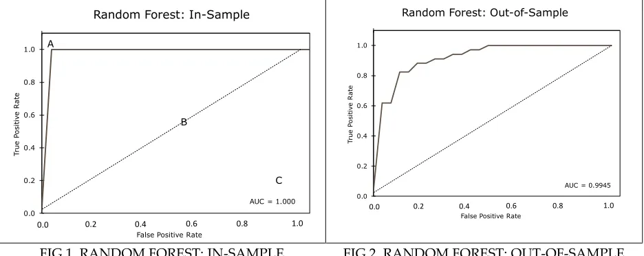
As mentioned earlier, the ROC AUC is utilized to measure a model’s performance. We estimated ROC AUC for all models and then compared them to select the best performing among the four models. The ROC curve along with an AUC for the random forest approach are plotted in Figure 1 (for in-sample analysis) and Figure 2 (for out-of-sample forecasts). A ROC curve, Figure 1, shows the plot of true positive rate (y-axis) against false positive rate (x-axis) at various threshold settings. The diagonal line (dotted line in Figure 1) is known as the line of no-discrimination, as an outcome on the line, point B for example, is almost as good as a random guess (probability of a true positive is equal to probability of a false positive). The area to the left of the diagonal line shows when the chance of a true positive rate is higher than the probability of a false positive rate at a given threshold. The left upper corner, point A for example, indicates the best possible prediction as it shows 100% accuracy. The right bottom corner, the corner closest to the point C, represents the worse possible prediction: a 100% chance of a false positive rate.
FIG 1. RANDOM FOREST: IN-SAMPLE FIG 2. RANDOM FOREST: OUT-OF-SAMPLE
The random forest in-sample analysis that produces an ROC AUVC value of one indicates the best in-sample fit. It is not a surprise that the random forest approach tends to produce a great in-sample fit. The out-of-sample forecasting simulations prove that the random forest approach is able to predict all recessions (1990, 2001 and 2007-2009 recessions) without producing a false positive as the ROC AUC is very close to one (0.9945), Figure 2. The random forest approach performance is excellent in both in-sample and out-of-sample simulations.
0.0 0.2 0.4 0.6 0.8 1.0 Tru e P o si ti ve R a te
False Positive Rate
Random Forest: In-Sample
AUC = 1.000
0.0 0.2 0.4 0.6 0.8 1.0
A B C 0.0 0.2 0.4 0.6 0.8 1.0 Tru e P o si ti ve R a te
False Positive Rate
Random Forest: Out-of-Sample
AUC = 0.9945
FIG 3. GRADIENT BOOSTING: IN-SAMPLE FIG 4. GRADIENT BOOSTING: OUT-OF-SAMPLE
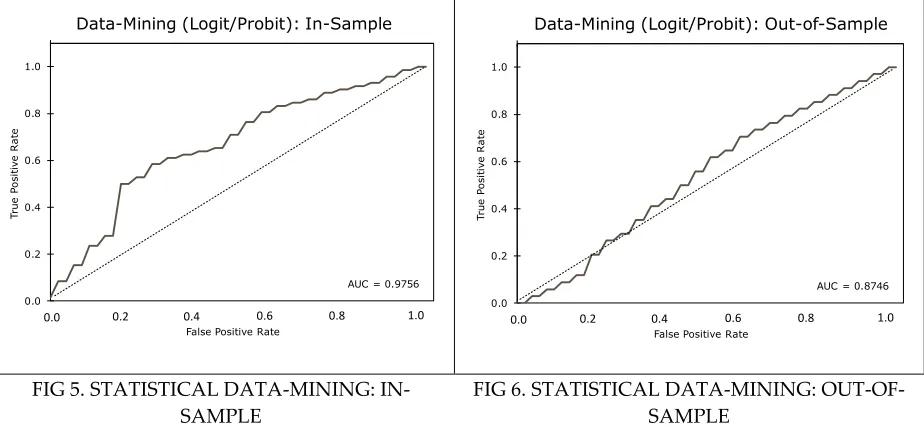
The results based on the gradient boosting are shown in Figure 3 (in-sample) and Figure 4 (out-of-sample). The in-sample AUC value is 1 and 0.9917 for the out-of-sample simulations. That is, the in-sample performance of the gradient boosting is equal to the random forest in-sample accuracy, but the random forest performed slightly better than the gradient boosting in the out-of-sample forecasting. The statistical data mining (logit/probit) approach came in at the third position with the ROC AUC value of 0.9756 (in-sample) and 0.8746 (out-of-sample) (Figure 5 & Figure 6).
FIG 5. STATISTICAL DATA-MINING: IN-SAMPLE
FIG 6. STATISTICAL DATA-MINING: OUT-OF-SAMPLE
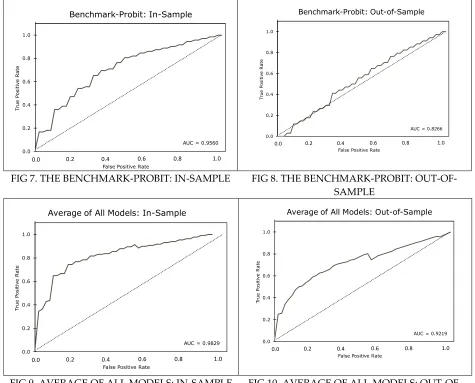
The benchmark probit model produces 0.9560 (in-sample) and 0.8266 (out-of-sample) values for the ROC AUC, the worst performer in our analysis (Figure 7 and Figure 8). The
0.0 0.2 0.4 0.6 0.8 1.0 Tru e P o si ti ve R a te
False Positive Rate
Gradient Boosting: In-Sample
AUC = 1.000
0.0 0.2 0.4 0.6 0.8 1.0
0.0 0.2 0.4 0.6 0.8 1.0 Tru e P o si ti ve R a te
False Positive Rate
Gradient Boosting: Out-of-Sample
AUC = 0.9917
0.0 0.2 0.4 0.6 0.8 1.0
0.0 0.2 0.4 0.6 0.8 1.0 Tru e P o si ti ve R a te
False Positive Rate
Data-Mining (Logit/Probit): In-Sample
AUC = 0.9756
0.0 0.2 0.4 0.6 0.8 1.0
0.0 0.2 0.4 0.6 0.8 1.0 Tru e P o si ti ve R a te
False Positive Rate
Data-Mining (Logit/Probit): Out-of-Sample
AUC = 0.8746
average of the all models are shown in Figure 9 and 10. The average of four models performed better than the benchmark and the data mining. However, the random forest and gradient boosting outperformed the average of all models. In addition, all four methods produce a very low probability (less than 5%) of a recession during the next 12 months.
FIG 7. THE BENCHMARK-PROBIT: IN-SAMPLE FIG 8. THE BENCHMARK-PROBIT: OUT-OF-SAMPLE
FIG 9. AVERAGE OF ALL MODELS: IN-SAMPLE FIG 10. AVERAGE OF ALL MODELS: OUT-OF-SAMPLE
Summing up, the evolution of big data and machine learning techniques open doors to improve economic/financial variables’ prediction. We believe that an effective modeling process can be dividing into two phases. The extraction of the useful information (signals vs. noises) is the first phase of an accurate modeling process and the second phase consists of utilizing that information efficiently (select appropriate estimation techniques). For example, in this analysis, we utilize the statistical data mining techniques to narrow down the FRED dataset (which contains more than 500,000 variables) to 192
0.0 0.2 0.4 0.6 0.8 1.0 Tru e P o si ti ve R a te
False Positive Rate
Benchmark-Probit: In-Sample
AUC = 0.9560
0.0 0.2 0.4 0.6 0.8 1.0
0.0 0.2 0.4 0.6 0.8 1.0 Tru e P o si ti ve R a te
False Positive Rate
Benchmark-Probit: Out-of-Sample
AUC = 0.8266
0.0 0.2 0.4 0.6 0.8 1.0
0.0 0.2 0.4 0.6 0.8 1.0 Tru e P o si ti ve R a te
False Positive Rate
Average of All Models: In-Sample
AUC = 0.9829
0.0 0.2 0.4 0.6 0.8 1.0
0.0 0.2 0.4 0.6 0.8 1.0 Tru e P o si ti ve R a te
False Positive Rate
Average of All Models: Out-of-Sample
AUC = 0.9219
variables. In other words, the data mining helps us to extract useful information (find signals and cancel noises).
In the estimation simulations, machine learning (the random forest and gradient boosting) techniques provided more accurate results using the same dataset than those of the logit/probit (statistical data mining) models. One major reason is that the logit/probit approach estimates an average relationship to predict an outcome. An average estimation process may limit the effectiveness of the modeling approach as relations between variables evolve overtime and the strength of the relationship fluctuates overtime as well. Machine learning techniques (both the random forest and gradient boosting) dig deeper and find useful statistical relationship between the target variable and predictors to generate forecasts. Therefore, both phases are necessary for accurate forecasting.
CONCLUDING REMARKS: IT’S NOT WHAT YOU HAVE, IT’S HOW YOU USE IT
The evolving nature of the economy forces decision makers to look for new tools to capture growing complexities in the economy to help them form effective policy. Our work proposes a new framework to generate accurate forecasts using a large set of predictors and machine learning tools. We stress that the extraction of useful information and the effective utilization of that information is crucial for accurate predictions.
The development of machine learning techniques along with large dataset availability opens doors to improving the predictive power of economic variables. We believe that an effective modeling process can be divided into two phases. The extraction of the useful information (signals vs. noises) first phase of an accurate modeling process. The second phase consists of utilizing that information efficiently.
variable and predictors to generate forecasts. Therefore, both phases are necessary for accurate forecasting.
Notes:
1Typically, an over-fitted model shows very good in-sample fit but very bad out-of-sample forecasts. For
more detail see, Silvia, J., Iqbal, A., et al. (2014). Economic and Business Forecasting: Analyzing and
Interpreting Econometric Results. Wiley 2014.
2The FOMC releases its meetings transcripts with a five year lag and can be found here:
https://www.federalreserve.gov/monetarypolicy/fomc_historical.htm
3It is worth mentioning that sometimes in machine learning/other big data applications different terms
(instead of in-sample and out-of-sample) are utilized such as training-sample or cross-validations etc. For more detail see, Hastie, T et al. (2008). The Elements of Statistical Learning. 2nd Edition, Springer. The basic logic behind all these procedures (analysis) is similar and that is to utilize some part of the available information (either time span, number of observations or both) to establish some statistical
association/relationship and then utilize those relationships to forecast future events (unknown values/outcome).
4For more detail about the FRED dataset see: https://fred.stlouisfed.org/
5If we use 1990-2005 period for in-sample analysis and rest of the period for out-of-sample simulation
then that will provide an opportunity to forecast only one recession and that recession is the Great Recession. That is not enough time span to test the real-time out-of-sample accuracy of a model.
6Note, for the Granger causality analysis, we utilize GDP growth rates as a target variable instead of a
binary variable (dummy variable to represent recession and non-recession periods). As the Granger causality test assumes the target variables are continuous not binary variables.
7For more detail about the Granger causality test see, Granger, C.W.J. (1969). Investigating Causal Relations
by Econometric Models and Cross-spectral Methods. Econometrica, 37(3).
8A p-value of less than or equal to 0.05 would reject the null hypothesis of no-causality and that indicates
the variable in the model is a good predictor of the target variable.
9For more detail about WoE and IV see, Lin, Alex. (2013). Variable Reduction in SAS by using Weight of
Evidence and Information Value. The full paper is available at: https://support.sas.com/resources/papers/ proceedings13/095-2013.pdf
10In simple words, if two (or more) predictors of a model are highly correlated with each other than that
issue is known as multi-collinearity. Typically, the multi-collinearity problem leads to an overfitting issue.
11For a detailed discussion about the ROC curve see, Lahiri, K., and J. G. Wang (2013). Evaluating
Probability Forecasts for GDP Declines Using Alternative Methodologies. International Journal of
Forecasting, 29, 175-190.
12For more details about machine learning applications in economics see Mullainathan, Sendhil and Jann
Spiess. (2017). Machine Learning: An Applied Econometric Approach. Journal of Economic Perspectives, 31(2).
13Breiman, Leo. (2001). Random Forests. Statistics Department, University of California, Berkeley, CA.
The paper is available at: https://www.stat.berkeley.edu/~breiman/randomforest2001.pdf
14Friedman, Jerome H. (1999). Greedy Function Approximation: A Gradient Boosting Machine. The full