33
Available online at http://ijdea.srbiau.ac.ir
Int. J. Data Envelopment Analysis (ISSN 2345-458X) Vol. 1, No. 1, Year 2013 Article ID IJDEA-00115, 10 pages
Research Article
Supplier Selection Using a DEA-TOPSIS Method
F.Ghaemi-Nasab*a,S.Mamizadeh-Chatghayehb
(a)Department of Mathematics, Andimeshk Branch, Islamic Azad University, Andimeshk, Iran (b)Young Researchers Club, Islamic Azad University, Central Tehran Branch, Tehran, Iran
Abstract
Supplier selection is one of the critical activities for firms to gain competitive advantage and achieve the objectives of the whole supply chain. In this paper based on a DEA-TOPSIS method for MADM problems a flexible strategy for supplier selection is introduced.
Keywords: Multiple criteria decision analysis, multiple criteria ranking, DEA, TOPSIS, supplier selection.
1 Introduction
Supply chain management (SCM) is one of the most important competitive strategies used by modern enterprises. Meanwhile, supplier selection plays an effective role in supply chain, [7]. Supplier selection problem is considered as a multiple attributes decision making (MADM) problem affected by several conflicting factors such as price, quality and delivery. Supplier selection requires the information about potential suppliers’ credit history, performance history and other personal information, which are often not available to the public, so that, strengthening partnerships with suppliers is most important for enhancing competitiveness, [12]. In the other word, supplier selection is evaluated as a critical factor for the companies desiring to be successful in nowadays competition conditions and order allocation are the most significant issues in the purchasing division of enterprises, [9], [13]. TOPSIS method that was developed by Hwang and Yoon (1981) is a famous useful method for MADM problems. This method is based on the concept that the chosen alternative should have the shortest Euclidean distance from the ideal solution, and the farthest from the negative ideal solution. The ideal solution is a hypothetical solution for which all attribute values correspond to the maximum attribute values in the database comprising the satisfying solutions; the negative ideal solution is the hypothetical solution for which all attribute values correspond to the minimum attribute values in the database. TOPSIS thus gives a solution that is not only closest to the hypothetically best, that is also the farthest from the hypothetically worst, [11]. Data envelopment analysis (DEA) is an increasingly popular managerial decision tool that was initially proposed by Charnes et al. in 1978. As a nonparametric method for estimating production frontiers, DEA measures relative performance of a set of producers or decision making units where the presence of multiple inputs and outputs makes comparisons difficult. During the last thirty years, significant research has been conducted on DEA for both theoretical extensions and practical applications, including various DEA-based MCDA approaches. A comprehensive survey of DEA among the early attempts of combining DEA with MCDA, [3], explore the utilization of
* Corresponding author, Email: [email protected]
efficiency analysis in DEA for evaluating alternatives in MCDA, [4], and suggests that cross efficiency-based DEA analysis could be a “Multi-attribute Choice (tool) for the Lazy Decision Maker: Let the Alternatives Decide!”. Stewart (1996) summarizes DEA and MCDA as “DEA arises from situations where the goal is to determine the productive efficiency of a system by comparing how well the system converts inputs into outputs, while MCDA models have arisen from the need to analyze a set of alternatives according to conflicting criteria.” A methodological connection between MCDA and DEA is that if “all criteria in an MCDA problem can be classified as either benefit criteria (benefits or output) or cost criteria (costs or inputs), then DEA is equivalent to MCDA using additive linear value functions” , [10]. In this paper using DEA-TOPSIS method, [1] a strategy for supplier selection is proposed. Since the TOPSIS method did not provide any relevant process to handle the uncertainty in ordinal criteria, this method adapts the method proposed by Cook & Kress, [1], [2] to address this problem. The DEA-TOPSIS method [1] provides a theoretically sound approach to quantifying qualitative criteria based on the aforesaid philosophy of individual performance optimization and so this method will be more reliable for supplier selection in real world. The remainder of the paper is organized as follows: Section 2 is allocated to the description of the concept of supplier selection, in section 3 the procedure of TOPSIS is introduced, section 4 is allocated to the DEA-TOPSIS [1] and finally as an application of DEA-TOPSIS method [1] a strategy for supplier selection is introduced.
2 Supplier Selection
One of the most important processes performed in enterprises today is the evaluation, selection and continuous measurement of suppliers. Also enterprise’s ability to produce a quality product at a reasonable cost and in a timely manner is heavily influenced by its suppliers’capabilities.
On the other hand, Supplier selection is one of the key issues of Supply Chain Management because the cost of raw materials and component parts constitutes the main cost of a product Management.
• Supplier Selection: “The stage in the buying process when the intending buyer chooses the preferred supplier or suppliers from those qualified as suitable.” (West burn Dictionary)
3 The Procedure of TOPSIS
The TOPSIS method is a distance-based approach, and its general procedure consists of the following steps [8]:
Step 1: Construct a performance matrix: An nq matrix contains the raw consequence data for all alternatives against all criteria as following:
A1 A2 ... An
1 11 12 1
2 21 22 2
1 2
... ...
... n
n
q q q qn
C y y y
C y y y
Y
C y y y
F.Ghaemi-Nasab et al /IJDEA Vol. 1, No. 1 (2013)33-42
A1 A2 ... An
1 11 12 1
2 21 22 2
2
1 2 1
... ... ; ... n n ij ij q ij
q q q qn i
C v v v
C v v v y
Y v
y
C v v v
Step 3: Define the ideal and anti-ideal point: Set the ideal point,
A
and anti-ideal point,A
, based on the normalized performance matrix. For a benefit criterion,Ci,
max 1n
i j ij
v A v and
min 1n
i j ij
v A v but for a cost criterion,Ck ,
min 1n
i j ij
v A v and vi
A maxnj1vij respectively.Step 4: Assign weights to criteria: Set
1
, 1
q
i i i
i w w Raanda w
to represent the relativeimportance of criterionCi. Note that R is the set of all real numbers.
Step 5: Calculate the distances of
A
j to the two ideal points,A
andA
: A commonly used distance definition is the Euclidean distance. Compute the distances of AjtoA
andA
usingEuclidean distance function,
21 q
j j
i i i
i
D A w v A v A
,
2 1 q j ji i i
i
D A w v A v A
Note that vi
Aj ,,
1 i q
, 1 j n
represents the i thelement of jth alternative vector.
Step 6: Obtain an integrated distance
A
j to these two extreme points: The distances ofA
j to the ideal and anti-ideal points have to be integrated to reach a final result. One way to integrate these two distances into an overall distance ofAj,D A
j , can be expressed as:
j j j j D A D AD A D A
where a larger value of D A
j represents a better overall performance.4 The DEA-TOPSIS method
In this section the method introduced in [1] is proposed. 4.1 Flexible Settings of
A
andA
Setting of ideal and anti-ideal points in the original TOPSIS is based upon value data that are normalized consequences reflecting the Decision-Makers' (DM's) preference directions over different criteria.
A
andA
are set as the combinations of either maximum or minimum values ofvi
Aj ,flexibility in setting
A
andA
, the approach reported in this method allows a DM to defineA
andA
in the consequence space directly with the following conditions: ,Aj A D A,,
j D A
: The normalized distance fromA
andA
should be larger than that between any alternative Aj in A andA
. ,Aj A D A,,
j D A
:The normalized distance fromA
andA
should be larger than that between any alternativeA
j in A andA
.To describe the distance definitions of different types of criteria more easily, let
C
C
cC
o,where C, Ccand Co represent the whole criteria set, quantitative (cardinal) criteria set and qualitative (ordinal) criteria set, respectively. Furthermore, let
1,, 2,...,,
c
c c c c
q C C C C and
1,, 2,...,, o
o o o o
q C C C C .
4.2 Definitions Over Cc
Let mic
Aj be the consequence measurement of Ajon a quantitative criterion, Cic. When, ,
j
A A or A, mic
Aj mic
A ,or m, ic
A . For eachCicCc, the distances from Aj to the predefined extreme points,A
andA
, are denoted as mic
A mic
Aj and
c c j
i i
m A m A , respectively. Then, an appropriate normalization function can be chosen to obtain the normalized distances of
A
j toA
andA
, denoted by dic
Aj anddic
Aj , respectively. In this paper vector-based normalization is used as detailed below. Note that in order to validate the two conditions in Section 4.1, the distance betweenA
andA
, mic
A mic
A , is included in the following normalization process. As a unique property of the new distance definitions, the following normalization function can be used over all kind of criterion (benefit, cost, or non-monotonic). There isn’t any require to explicitly differentiate these three types of criteria in this normalization. Vector-based normalization [1]:
2
21 n
c c j c c
i i i i i
j
m A m A m A m A
as the ideal normalization factor, and
2
21
n
c c j c c
i i i i i
j
m A m A m A m A
as the anti-ideal normalization factor. Then, the normalized distance between
A
j
A
andA
over criterion Ciis defined as:
ic
ci
jc j
i
i
m A m A
d A
F.Ghaemi-Nasab et al /IJDEA Vol. 1, No. 1 (2013)33-42
ic
ci
jc j
i
i
m A m A
d A
By plugging
A
in dic
. andA
in dic
. we have:
ic
ic
c i
i
m A m A
d A
,
c c i i c i im A m A
d A
4.3 Definitions Over Co
Nowadays linguistic terms are commonly used for measuring consequences over qualitative criteria, o
C . Let L
l l1, 2,...,lm
as the linguistic terms set, where l1 represents the best level, l2 the next best, …, and lmthe worst grade. Then, mio
Aj lr means thatA
j has the grade lrover criterion. Since the linguistic grade set represents a preference order, obviously,
1o i
m A l and
o
i m
m A l , because the linguistic grade for
A
on criterion o iC should be the best one, l1, and in the same way the grade of
A
should be the worst, lm. Now suppose that
o j
i
d A anddio
Aj represent the distance betweenA
j andA
, and betweenA
j andA
over the criterion Cio, respectively. Similar to qualitative criterion case distances should be normalized to between 0 and 1, in this paper we supposed that the distance betweenA
j andA
over Ciois 1,(dio
A dio
A 1). Using piecewise linear interpolation, if mio
Aj lr, then we have the following conditions: , r 1 dio
Aj rm m
, and m r 1 dio
Aj m rm m
.
After obtaining the normalized distances from each alternative
A
j toA
andA
, an aggregated distance related to the so-called p-norm, where p ≥ 1 , will be used to obtain the integrated normalized distances, di
A j and di
Aj , over each criterion. The norms p=1 and p=2 are most used. If
1, 2,... ,. c
c c c c
q
w w w w and
1, 2,... ,.
o
o o o o
q
w w w w represent the weight information for Ccand o
C respectively Then, the weighted p -power distance of
A
j toA
over CcandCowill be
1
1 1
. . 4 1
c o
p
q p q p
j c c j o o j
j i j i
i i
D A w d A w d A
and
1 1 1. . 4 2
c o p
q p q p
j c c j o o j
j i j i
i i
D A w d A w d A
Obviously, when
A
j
A
, D A
j D A
and D A
j D A
forA
j
A
.4.4 Imprecise Intrinsic Preference Expressions
4.5 A DEA-based Model
Before adopting TOPSIS method the parameters, w c, wo, djo
Aj anddjo
Aj , ,CioCoand jA
A
, should be obtained. In this paper the following optimization is used for this purpose:
, ,,,,,,,,,,,,,,,,,,,,,,,,,,,,,,,,,,,,,,, ,,,,,,,,,,,,,,,,,,,,,,,,,,,,,,,,,,,,,,,, ,,,,,, ,,,,,,,,,,,,,,,,,,,,,,,,,,,,,,,,,,,,,,,, ,,,,,,,,,,,,,,,,,,,,,,,,,,,,,,,,,,,,,,,, ,,,,,,,, m , ax , . ,,, j j j D AD A D A
s t
,,,,,,,,,,,,,,,,,,,,,,, , ,, ,,,,,,,,,,,,,,,,,,,,,,,,,,,,,,,,,,,,, ,,,,,,,,,,,,,,,,,,,,,,,,,,,,,,,,,,,,,,, , ,, ,,,,,,,,,,,,,,,,,,,,,,,, , 1 ,, ;, 1; ,,,,,,,,,,, 4 3 ,,,,,,,,,,,,,,,,,,,
j j
j j
A A D A D A
A A D A D A
,,,,,,,,,,,,, , , , , , , , ,,,,,,,,,,, , , ,,,,,,,,,,,,,,,,,,,,,,,,,,,,,,,,,,,,,, ,,,,,,,,,,,,,,,,,,,,,,,,,,,,,,,,,,,, 1 ,,,,,,,,,,,,,,, 1 , , ; ; , , 1j o j o j o j
j r j j
o o o
i i
i
r r m r m r
A A if m A l then d A and d A
m m m m
C C d A
C
oCo,,dio
A 1;,,,,,,,,,,,,,,,,,,,,,,,,,,,,,,,,,,,,,,, ,,,,,,,,,,,,,,,,,,,,,,,,,,,,,,,,,,,,,,,, ,,,,,,,,,,1 1 ,,,,,,,,,,,,,,,,,,,,,,,,,,,,,,,,, , , ,, ,, 1; , , ,, c o q q c o i i i i
c c c o o o
i i i i
w w
C C w and C C w
Note that the two conditions of setting
A
andA
in Section 4.1 have to be verified. 5 Supplier Selection Using DEA-TOPSIS methodIn this section our proposed strategy for supplier selection is introduced. Let n supplier and q attributes there exist:
Step1. Construct the decision matrix Y.
Step2. Construct the weights order as mentioned in 4.4 and obtain equivalent constraints. Step3. Obtain Positive Ideal Supplier (PIS) and Negative Ideal Supplier (NIS).
Step4. Using (4-2) and (4-3) and Feeding constraints obtained in Step2 in to the optimization model (4-5) obtain the relative closeness between each supplier and ideal suppliers.
Step5. Order the suppliers with respect to their relative closeness obtained in previous step, the larger the higher efficiency and subsequently lower ranking order.
F.Ghaemi-Nasab et al /IJDEA Vol. 1, No. 1 (2013)33-42
6 Numerical example
In this section an illustrative numerical example [1] is introduced. Let eight suppliers, Sj, 1,
j 8
, and seven attributes (all of them are cost attributes) there exist. The basic structure of problem is introduces in table 6.1 and the weights orders are as follows:1 2 3
c c c
w w w , w1c w2c w4c, w1c w5c, w6c w1o
To strengthen the expression of “preferred” or “more important”, it is assumed that the weight gap between the above inequalities is greater than or equal to 0.1, hence the above preference relationships can be translated into the following constraints:
1 2 0.1
C C
w w , w2C wC3 0.1, w1C wC4 0.1, wC2 wC4 0.1, w1C w5C 0.1,
6 1 0.1
C o
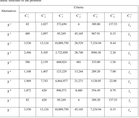
w w Table 6.1
Basic structure of the problem
Alternatives
Criteria
1
c
C C2c C3c C4c C5c C6c C1o
1
S 82 1,027 372,650 6 389.80 137.53 l4
2
S 489 1,097 85,249 45,165 967.91 0.15 l4
3
S 3,530 13,124 10,009,750 28,529 7,234.94 8.44 l1
4
S 2,496 5,105 2,722,850 28,740 3096.30 2.26 l2
5
S 386 2,139 668,024 681 333.00 1.56 l3
6
S 1,108 1,407 123,229 13,244 289.20 7.08 l3
7
S 1,969 7,743 6,864,977 21,271 1128.05 22.00 l2
8
S 1,872 620 896,571 8,460 554.49 0.79 l3
S 82 620 85,249 6 289.20 137.53 l1
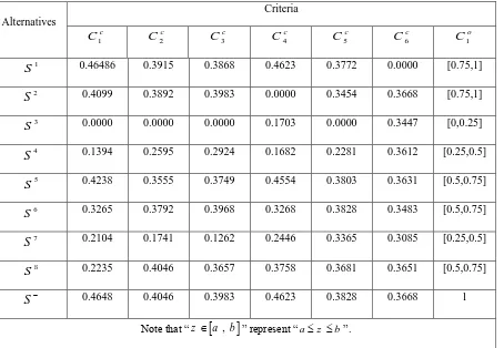
Table 6.2
Normalized distance information to S Alternatives
Criteria
1
c
C C2c C3c C4c C5c C6c C1o
1
S 0.46486 0.3915 0.3868 0.4623 0.3772 0.0000 [0.75,1]
2
S 0.4099 0.3892 0.3983 0.0000 0.3454 0.3668 [0.75,1]
3
S 0.0000 0.0000 0.0000 0.1703 0.0000 0.3447 [0,0.25]
4
S 0.1394 0.2595 0.2924 0.1682 0.2281 0.3612 [0.25,0.5]
5
S 0.4238 0.3555 0.3749 0.4554 0.3803 0.3631 [0.5,0.75]
6
S 0.3265 0.3792 0.3968 0.3268 0.3828 0.3483 [0.5,0.75]
7
S 0.2104 0.1741 0.1262 0.2446 0.3365 0.3085 [0.25,0.5]
8
S 0.2235 0.4046 0.3657 0.3758 0.3681 0.3651 [0.5,0.75]
S 0.4648 0.4046 0.3983 0.4623 0.3828 0.3668 1
Note that “z
a, ,,b
” represent “az b ”.Table 6.3
Normalized distance information to S Alternatives
Criteria
1
c
C C2c C3c C4c C5c C6c C1o
1
S 0.0000 0.0207 0.0181 0.0000 0.0098 0.7015 [0,0.25]
2
S 0.0663 0.0243 0.0000 0.5637 0.0660 0.0000 [0,0.25]
3
S 0.5617 0.6357 0.6264 0.3561 0.6759 0.0423 [0.75,1]
4
S 0.3933 0.2280 0.1665 0.3587 0.2731 0.0108 [0.5,0.75]
5
S 0.0495 0.0772 0.0368 0.0084 0.0043 0.0072 [0.25,0.5]
6
S 0.1671 0.0400 0.0024 0.1653 0.0000 0.0354 [0.25,0.5]
7
S 0.3074 0.3621 0.4279 0.2655 0.0816 0.1116 [0.5,0.75]
8
F.Ghaemi-Nasab et al /IJDEA Vol. 1, No. 1 (2013)33-42
S 0.5617 0.6357 0.6264 0.5637 0.6759 0.7015 1
Note that “za, ,,b” represent “a z b”.
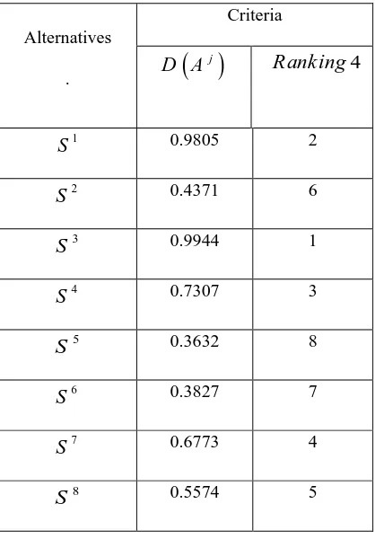
Table 6.4
Final distance performance and rankings
Alternatives .
Criteria
jD A
Ranking4
1
S 0.9805 2
2
S 0.4371 6
3
S 0.9944 1
4
S 0.7307 3
5
S 0.3632 8
6
S 0.3827 7
7
S 0.6773 4
8
S 0.5574 5
7 Conclusions
Considering the fact that one of the most important processes performed in enterprises today is the evaluation, selection and continuous measurement of suppliers, in this paper a hybrid DEA-TOPSIS method was introduced for supplier selection. Since proposed supplier selection method uses DEA in selection process and considers the fact that in practice, a DM may often have ideal or anti-ideal alternatives (points) directly on consequences, rather than on normalized values, it is a flexible manner which evaluates and selects suppliers.
References
[1] Chen, Y., Kevin, W.LI.,&Xu, H., &Liu,S. A DEA-TOPSIS method for multiple criteria decision analysis in emergency management, Journal of Systems Sciences and Systems Engineering, 18(4): 489-507, (2009).
[3] Doyle, J., & Green, R. Efficiency and cross-efficiency in DEA: derivations, meanings and uses. Operational Research Society, 45: 567-578, (1994).
[4] Doyle, J. Multi-attribute choice for the lazy decision maker: let the alternatives decide! Organizational Behavior and Human Decision Processes, 62: 87-100, (1995).
[5] Eum, Y.S., Park, K.S. &Soung, S.H. Establishing dominance and potential optimality in multi-criteria analysis with imprecise weight and value. Computers and Operations Research, 28: 397-409, (2001).
[6] Sage, A.P. & White, C.C. ARIADNE: a knowledge-based interactive system for planning and decision support. IEEE Transactions on Systems, Man and Cybernetics, 14: 35-47, (1984).
[7] Shahanaghi, K. Yazdian, S.A. Vendor selection using a new fuzzy group TOPSIS approach. Journal of Uncertain Systems, 3.221-231, (2009).
[8] Shih, H.S., Shyur, H.J., & Lee, E.S. An extension of TOPSIS for group decision-making. Mathematical and Computer Modeling, 45: 801- 813, , (2007).
[9] Simpson, P.M., Siguaw, J. A., & White, S. C. Measuring the performance of supplier: An analysis of evaluation processes, Journal of Supplychain Management, 38, 29-41, (2003).
[10] Stewart, T. Relationships between data envelopment analysis and multi- criteria decision analysis. Journal of the Operational Research Society, 47: 654-665, (1996).
[11] V.Rao, Decision-making in the manufacturing environment: Using graph theory and fuzzy multiple attributes decision-making methods. India: Springer series in advanced manufacturing, (2007).
[12] Wu, D. (2009). Supplier selection: A hybrid model using DEA, decision tree and neural network. Expert Systems with Applications, 36: 9105–9112, (2009).