BMC Medical Research Methodology
2002, 2
Research article
Markers for early detection of cancer: Statistical guidelines for
nested case-control studies
Stuart G Baker*
1
, Barnett S Kramer
2
and Sudhir Srivastava
1
Address: 1Division of Cancer Prevention, National Cancer Institute, Bethesda, MD, USA and 2Office of Disease Prevention and Medical
Applications of Research, National Institutes of Health, Bethesda MD, USA
E-mail: Stuart G Baker* - [email protected]; Barnett S Kramer - [email protected]; Sudhir Srivastava - [email protected] *Corresponding author
Abstract
Background: Recently many long-term prospective studies have involved serial collection and storage of blood or tissue specimens. This has spurred nested case-control studies that involve testing some specimens for various markers that might predict cancer. Until now there has been little guidance in statistical design and analysis of these studies.
Methods: To develop statistical guidelines, we considered the purpose, the types of biases, and the opportunities for extracting additional information.
Results: The following guidelines:
(1) For the clearest interpretation, statistics should be based on false and true positive rates – not odds ratios or relative risks
(2) To avoid overdiagnosis bias, cases should be diagnosed as a result of symptoms rather than on screening.
(3) To minimize selection bias, the spectrum of control conditions should be the same in study and target screening populations.
(4) To extract additional information, criteria for a positive test should be based on combinations of individual markers and changes in marker levels over time.
(5) To avoid overfitting, the criteria for a positive marker combination developed in a training sample should be evaluated in a random test sample from the same study and, if possible, a validation sample from another study.
(6) To identify biomarkers with true and false positive rates similar to mammography, the training, test, and validation samples should each include at least 110 randomly selected subjects without cancer and 70 subjects with cancer.
Conclusion: These guidelines ensure good practice in the design and analysis of nested case-control studies of early detection biomarkers.
Published: 28 February 2002
BMC Medical Research Methodology 2002, 2:4
Received: 2 October 2001 Accepted: 28 February 2002
This article is available from: http://www.biomedcentral.com/1471-2288/2/4
Background
Most current methods of cancer early detection, such as mammography or cervical cytology, are based on anatom-ic changes in tissues or morphologanatom-ic changes in cells. Re-cently, various molecular markers, such as protein or genetic changes have been proposed for cancer early de-tection [1–4]. This has spurred many investigators with long-term cohort studies to serially collect and store blood or tissue specimens. The aim is to later perform a nested-case control study, where specimens from subjects with a particular type of cancer (cases) and specimens from a random sample of subjects without the cancer (controls) are tested for various molecular markers. Sometime this sort of study is called a retrospective longitudinal study [6] although retrospective longitudinal data could arise in other ways, as well. Unlike cross-sectional study designs, the markers are measured on specimens collected well be-fore the onset of clinical disease in cases. This avoids the potential confounding effect of the target disease on the marker.
For example, in the ATBC (alpha-tocopherol, beta-caro-tene) [7] and CARET [8] studies, subjects were rand-omized to placebo or drug to in a long-term study to determine the effect of the drug on lung cancer mortality. During the course of the trial serum was serially collected and stored in a biorepository. In a subsequent nested case-control study, stored serum samples from all cases of pros-tate cancer and a random sample of controls were tested for prostate-specific antigen (PSA).
Importantly the nested case-control study of early detec-tion biomarkers may be distinct from the original long-term study from which serum were collected. It is de-signed to answer a different question, it typically studies subjects with a different disease, and it often ignores the intervention in the original long-term study.
Methods
We had three considerations in formulating appropriate guidelines. First we wanted to link the analysis to the goal of study, namely, to help decide on further study of the bi-omarker as a trigger for early intervention. Second we wanted to minimize possible biases in the selection of cas-es and the controls and in the invcas-estigation of many mark-ers. Third, we wanted to extract as much information as possible relevant to the evaluation.
Results
We offer the following guidelines for the design and anal-ysis of nested case-control studies of early detection cancer biomarkers.
1. For the clearest interpretation, statistics for binary markers should be based on true and false positive rates
or predictive values based on the true prevalence – not odds ratios, relative risks, or predictive values based on the prevalence in the study
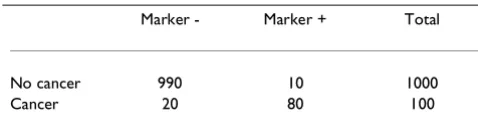
A promising marker should have a high degree of accuracy in discriminating between subjects who are likely to get cancer from those who are not. For a binary marker, which is either positive or negative, the basic measures of this type of accuracy are the true positive and false positive rates. Consider the hypothetical data in the Table 1 from a nested case-control study of early detection biomarkers. The true positive rate (TPR), or the test sensitivity, is the probability the marker is positive given cancer. The false positive rate (FPR), or 1 – specificity, is the probability the marker is positive given no cancer. In Table 1, TPR is esti-mated by 80/100 = .80, and FPR is estiesti-mated by 10/1000 = 01. For a perfect test, TPR = 1 and the FPR = 0. There is always a tradeoff between the TPR and FPR, so it is mean-ingless to assess one without assessing the other. For ex-ample, one could make the TPR equal to 1 simply by classifying every subject as positive for cancer. But this would be a poor classification rule because the FPR would also be 1.
Guidelines for FPR and TPR
Because the underlying prevalence of cancer is so low in average risk populations, for acceptable cancer screening of asymptomatic people, the FPR should be very small [9]. As a starting point we recommend basing guidelines for FPR and TPR on the FPR and TPR for mammography, which, as discussed below, is FPR=.01 and TPR=.80. A mammogram is analogous to a biomarker test for cancer but there is extra information from various studies that makes it useful for setting guidelines.
One reason for using FPR and TPR from mammography as a standard is that, unlike biomarker measurements in nested case-control studies, in mammography studies there is a biopsy at the time of a positive test. This biopsy is the gold standard for determining cancer status in sub-jects with positive mammograms and is used for
comput-Table 1: Hypothetical data for a binary marker from a nested case-control study
Marker - Marker + Total
No cancer 990 10 1000
Cancer 20 80 100
ing TPR in a way not possible with biomarkers in nested case-control studies. The TPR for mammography is the probability of a positive biopsy as a direct result of mam-mography in women with cancer and is estimated via mathematical models or data collected after following subjects not biopsied. As discussed in Baker and Pinsky [10], estimates ranged from .74 to 1.00 with .80 a conserv-ative value.
Importantly the estimated TPR for mammography is not likely to be affected by overdiagnosis, which means that some screening-detected cancers would never have caused medical problems during the patient's life [11]. This would make the biomarker appear more promising than actually the case. Results from the HIP screening trial of mammography and clinical self-examination [12] suggest that if there were overdiagnosis with mammography, it would be relatively small. At the time of the last breast screening in the HIP trial, there were more cancers in the group randomized to screening than in the controls. But with further follow-up the number of cancers in the con-trol group eventually equaled the number in the screened group, which would not have occurred if there were sub-stantial overdiagnosis.
A second reason for using FPR and TPR from mammogra-phy is that, based on various randomized trials with can-cer mortality endpoint, mammography is generally considered an acceptable screening modality. The impli-cation is that a similar FPR and TPR for a biomarker would lead to an acceptable screening modality. For a particular biomarker, these target values of FPR and TPR from mam-mography may need modification depending on various factors. One factor is the invasiveness of a follow-up pro-cedure to investigate a positive test (e.g. needle biopsy of the prostate to investigate an abnormal PSA versus laparotomy to investigate an abnormal CA125). The more invasive the follow-up procedure, the lower the FPR must be to gain acceptance in practice. A second factor is addi-tional work-up prior to a biopsy. If a positive biomarker is unlikely to trigger additional diagnostic work-ups prior to biopsy, a higher FPR might be acceptable.
One caveat when using FPR from mammography is to be careful as to its definition. The restricted definition is the probability of a positive biopsy as a direct result of mam-mography in women without cancer. The less restricted definition is the probability of a suspicious mammogram warranting additional diagnostic follow-up of any type in women without cancer. Typically nested-case control studies of early detection biomarkers do not provide in-formation on additional diagnostic follow-up. Therefore they cannot be used to estimate a less restricted FPR in-volving diagnostic follow-up. However, because nested case-control biomarker studies provide data on cancer
di-agnosis, they can be used to estimate a more restricted FPR based on unnecessary biopsies. Therefore the target FPR is based on the more restricted definition of FPR in mam-mography. For mammography the more restricted FPR is estimated by the fraction of women screened by mam-mography who received a biopsy in which no cancer was detected. As discussed in Baker and Pinsky [10], estimates of FPR from three studies ranged from .005 to .013 with a middle value of around .010.
Inappropriateness of odds ratio and relative risk
When evaluating binary early detection markers, it is inap-propriate to report an odds ratio or relative risk, as is com-mon in epidemiology or clinical trials. Because an odds ratio or relative risk is a single number, it does not capture the tradeoff between correctly classifying cancer and in-correctly classifying non-cancers. Also the odds ratio or relative risk can lead to an overoptimistic impression of the performance of an early detection test if the interpre-tation is based on experience in epidemiology or clinical trials. In the latter settings an odds ratio of 3 is often con-sidered large. Much larger odds ratio are needed from ear-ly detection tests for useful application in the screening setting [13]. For example, for the target values of FPR = .01 and TPR = .80, the odds ratio equals (TPR × (1-FPR)/ ((1-TPR) × FPR) = 396, as in Table 1.
Appropriate computation of predictive values
It is sometimes useful to use the FPR and TPR to compute the predictive value negative (PVN), the probability of no disease if the marker is negative, and the predictive value positive (PVP), the probability of disease if the marker is positive. For cancer screening, it is the PVP that is most im-portant to the physician in clinical decision-making. Be-cause the likelihood of any individual cancer type in an asymptomatic person is nearly always very low, a negative early detection test usually adds little information to the clinical impression. The computation of the PVN and PVP depend on the prevalence of cancer as well as on the FPR and the TPR, as shown below,
PVP = (TPR × prevalence) / (TPR × prevalence + FPR (1-prevalence))
PVN = (1-FPR) × (1-prevalence) / ((1-TPR) × prevalence + (1-FPR) (1-prevalence))
ex-ample suppose FPR = .01, TPR = .80, and prevalence = .003. We obtain,
PVP = = (.8 × .003) /(.8 × .003 + .01 .997)= .19
PVN = (.99 × .997) / (.2 × .003 + .99 × .997) = .999
If we had incorrectly substituted the apparent prevalence in Table 1 of 100/1100 = .091, we would have incorrectly computed PVP = .89 and PVN = .980. For this reason, cal-culation and reporting of PVP and PVN using only data from a nested case-control study is not useful or appropri-ate.
Extension to ordered categories via ROC curves
Many markers for the early detection of cancer can be re-ported as ordered categories. Some markers, such as spu-tum cytology, inherently involve ordered categories, such as no evidence of cancer, slight atypia, moderate atypia, severe atypia, and frank cancer. Other markers, such as PSA, involve a continuous measure for which higher val-ues indicate a greater probability of cancer. Dividing these continuous measures into ranges (either based on prede-termined values or percentiles) gives ordered categories.
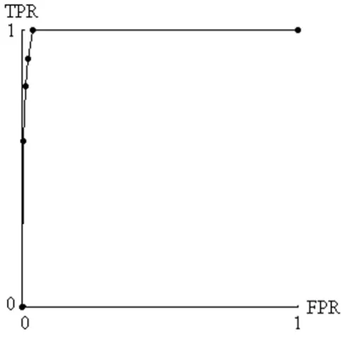
With ordered categories, the statistics should still be based on FPR and TPR. Each ordered category is a possible cut-point, where values equal to or higher than the cutpoint are called positive and values lower than the cutpoint are called negative. For each cutpoint, one can compute FPR and TPR (Table 2) and generate a receiver-operating char-acteristic (ROC) curve, which is a plot of TPR versus FPR for the various pairs [14]. (See Figure 1). The higher and farther left the points on the ROC curve the better the test performance. As mentioned previously, acceptable cancer screening requires very small false positive rates. There-fore, for evaluating cancer biomarkers, we are only inter-ested in the leftmost sliver of the ROC curve in Figure 1.
2. To avoid overdiagnosis bias, cases should be diag-nosed as a result of symptoms rather than on screening
For the TPR in the biomarker study to reflect the true TPR, cases should be diagnosed as a result of symptoms rather than on screening. For example in the study of PSA in the ATBC trial [7], cases were subjects diagnosed with prostate cancer as a result of symptoms. If the prostate cancer cases were detected as the result of screening, say with ultra-sound, the TPR could be artificially elevated if there were overdiagnosis, as previously discussed.
3. To minimized selection bias, the spectrum of control conditions should be the same in study and target screening populations
For the FPR in the nested case-control study to reflect the true FPR in the target population, the spectrum of control conditions should be the same as in the target population. By control conditions, we mean characteristics of the pop-ulation, such as the presence of other diseases or certain known risk factors that could elevate the false positive rate.
The spectrum of conditions could differ considerably if the retrospective biomarker study were embedded in a
Table 2: Hypothetical Data for an Ordered Marker From a Nest-ed Case-Control Design
1 2 3 4 5
No cancer 960 20 10 8 2 1000
Cancer 0 10 10 20 60 100
For cutpoint 4, the true positive rate is (20+60)/100 = .80 For cut-point 4, the false positive rate is (8 + 2)/1000 = .01
Figure 1
randomized trial with strict eligibility requirements. For example, consider a biomarker for the early detection of lung cancer where the data comes from a biorepository arising from a randomized trial of healthy subjects. It would be inappropriate to apply the results to a popula-tion with a high prevalence of chronic obstructive lung disease, bronchitis, or viral pnuemonitis because these conditions could increase the number of positive readings in subjects without lung cancer. Because FPR is very small for screening to be acceptable, this spectrum bias could have important consequences in a clinical application.
It would not always be possible to identify all relevant control conditions, but to the extent possible, the control conditions should be similar in both populations.
4. To extract additional information, criteria for a posi-tive test should be based on combinations of individual markers and changes in marker levels over time
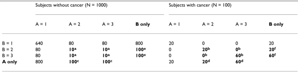
Data from multiple markers present an opportunity to ex-tract potentially valuable information not available by an-alyzing markers separately. Consider the hypothetical data in Table 3. The left side corresponds to subjects with-out cancer, and the right corresponds to subjects with can-cer. In our idealized circumstance, markers A and B are independent for subjects without cancer and are perfectly correlated for subjects with cancer. The indicated region for A = 2 or A = 3 and B = 2 or B = 3 designates a positive test that has FPR = .04 and the TPR = .80. Suppose that marker A and marker B were evaluated separately. The in-dicated region corresponding to A only, namely A = 2 or A = 3 and the indicated region corresponding to B only, namely B = 2 and B = 3, each designates a positive test that has FPR=. 20 and TPR=. 80. Thus, in this particular exam-ple, the combination of markers leads to a much better test than the separate markers, with a smaller FPR (.04
ver-sus .20) for the same TPR of .80. One could create a simi-lar example with any number of marker levels. For an ideal test in which FPR = 0 and TPR = 1, the region would encompass all subjects with cancer but no subjects with-out cancer.
A real application of how marker combinations provide extra information comes from a recent study by Mok et al [15] on CA125 and Prostasin as markers for ovarian can-cer. Although the data are not from a nested case-control study and have not been validated in subsequent studies, they are useful for illustration. Based on Figure 5 of Mok et al [15] with approximate values for the outpoints, we investigated regions with FPR=.02. The combination for a positive test of CA 125 greater than or equal to 40 U/ml and Prostasin greater than or equal to 5 µg/ml had FPR = .02 and TPR = .92. Evaluating CA 125 alone, the criterion for a positive test of CA 125 greater than 80 U/ml had FPR=.02 and TPR =.78. Evaluating Prostasin alone, the cri-terion for a positive test of Prostasin greater than 15 µg/ml had FPR=. 02 and TPR=. 32. Thus, in this real example, the combination of markers led to a better test than the sepa-rate markers, with a larger TPR (.92 versus .78 or .32) for the same FPR of .02.
To more generally compare performance of a combina-tion of markers with a single marker, we need to compare ROC curves. Creating an ROC curve from a combination of markers is different from creating an ROC curve from a single marker. With a combination of markers, the number of possible regions, as in Table 3 a, for calling a marker positive is extremely large. Some choices of re-gions correspond to AND rules, for example A>1 and B>1, as in Table 3 a. Some choices of regions correspond to OR rules, for example A>2 or B>2. Other choices are also pos-sible, but for biological reasons, one would usually re-quire all regions to be contiguous. A plot of the FPR and
Table 3: Hypothetical data for two ordered markers, A and B
Subjects without cancer (N = 1000) Subjects with cancer (N = 100)
A = 1 A = 2 A = 3 B only A = 1 A = 2 A = 3 B only
B = 1 640 80 80 800 20 0 0 20
B = 2 80 10a 10a 100e 0 20b 0b 20f
B = 3 80 10a 10a 100e 0 0b 60b 60f
A only 800 100c 100c 20 20d 60d
For A and B combined; aFalse positive rate (FPR) of indicated region (10+10+10+10)/1000=. 04; bTrue positive rate (TPR) of indicated region =
(20 +0+0+60)/100=. 80 For A only; cFalse positive rate (FPR) of indicated region =(100+100)/1000=. 20; dTrue positive rate (TPR) of indicated
region = (20+60)/100=. 80 For B only; eFalse positive rate (FPR) of indicated region =(100+100)/1000= .20; fTrue positive rate (TPR) of indicated
TPR for each region would lead to a cloud of points, rather than the smooth curve in Figure 1. To create the best ROC curve, one should select those points that are highest and farthest to the left, which is generally all that would need to be presented and only for small false positive rates. For complicated situations, Baker [16] proposed an algorithm to select the regions creating the best ROC curve without the need to enumerate all the regions. Mathematically, in any sample of data, the best ROC curve for a combination of markers must be as good or better than the ROC curve for any of the markers evaluated separately. The reason is that the set of possible regions for calling a combination of markers positive includes as a special case the regions for calling any single marker positive.
Alternative approaches that do not directly optimize the ROC curve include linear logistic regression or linear dis-criminant analysis [17], which choose regions based on linear combinations of the markers, and neural networks [18], which choose regions in a very complicated nonlin-ear manner. Due to the potential for overfitting (to fol-low), it is not possible to make a blanket statement as to which approach for choosing regions is best. If one takes the set of regions for calling a combination positive that gives a good ROC curve in a random sample of data, it may give a poor ROC curve in another random sample of the data, simply due to selecting chance patterns in the first sample. As discussed in the section on overfitting, this motivates splitting the data into two random samples, training and test, and using the regions from the training sample to compute the definitive ROC curve based on data in the test sample.
Changes in marker values over time also provide poten-tially valuable information not available when examining markers at a single time point. With marker measure-ments at two different times per subject (and approxi-mately the same interval between times), a common summary measure is the slope. If investigators believe that both slope and baseline level predict cancer, the combina-tion can be evaluated using the previously discussed methods for evaluating multiple markers, namely, treat-ing baseline level and slope as two "separate" markers. With measurements at more than two times per subject, investigators may identify a more complicated feature, such as whether or not there is a sudden increase in mark-er levels [19].
When biomarker measurements occur at regular time in-tervals (and allowing different numbers of measurements for each subject), one can estimate TPR and FPR by using a first order Markov chain in reverse time, as described by Baker and Tockman [20] for the analysis of precancerous lesions for lung cancer.
5. To avoid overfitting, the criteria for a positive marker combination developed in a training sample should be evaluated in a random test sample from the same study and, if possible, a validation sample from another study.
With a single marker and a large number of subjects, there is usually no concern with overfitting. However with many combinations of markers, overfitting could invali-date results. Overfitting is often associated with step-wise regression models [21] but it can occur in other situations as well. Overfitting of a larger number of markers to a rel-atively small number of subjects produces a model that is overly sensitive to chance fluctuations in the data. As a simple example, overfitting occurs when a sports an-nouncer reports that a baseball player had a very high bat-ting average against left-handed pitchers in ballpark X over the past month. This average is not very reliable for future predictions because the particular set of factors, left-handed pitchers and ballpark X, were selected to give a high average. In reality the high average is more likely the result of chance factors that coincided with left hand-ed pitchers at ballpark X during that particular month. One way to adjust for overfitting is to apply the factors in another sample not used for initial reporting. The first sample is known as the training sample, and the second sample is known as the test sample. For example, the pre-diction of the average against left handed pitchers in the ballpark X could be tested on data from a different month. Similarly, a standard statistical approach to adjust for overfitting is to randomly split the data into a training and test samples. This is called the split-sample approach. Promising marker combinations are identified in the training sample, but more reliable FPR and TPR measure-ments are made in the test sample because it involves dif-ferent data. Baker [16] used the split-sample approach to evaluate the performance of four markers for prostate can-cer.
and (iii) the statistics from each resampling are combined in a special way [22]. In a recent study comparing these adjustments with other types of statistics in a different set-ting, Steyerberg et al [22] found that the split-sample ap-proach tended to underestimate performance, cross-validation performed poorly on some statistics that were not normally distributed, and bootstrapping performed best overall. For our purposes of estimating an entire ROC curve rather than a summary statistic, more research is needed for cross-validation and bootstrapping, as it is not clear how best to combine ROC curves over different sam-ples.
Regardless of the method used to adjust for overfitting in forming a classification rule, to obtain the most reliable FPR and TPR measurements, the classification rule should ideally be evaluated in a validation sample from a different
study, as in Baker [16].
6. To identify biomarkers with true and false positive rates similar to mammography, the training, test, and validation samples should each include at least 110 ran-domly selected subjects without cancer and 70 subjects with cancer (as based on FPR and TPR for mammogra-phy)
The sample size is based on the need to determine if the biomarker is sufficiently promising for investigation as a trigger for early intervention in a future trial. As discussed previously, based on considerations from mammography, our target values are FPR = .01 and TPR= .80. In most sit-uations, we think it would be of interest to specify a 95% confidence interval for TPR of (.70, .90). Using a normal approximation the target standard error is approximately .05. Setting the standard error of TPR, TPR × (1-TPR) / (square root of n), equal to .05 and solving for the sample size n, we obtain n= 64, which we round up to 70. In ad-dition we think that in most situations the largest reason-able value of FPR would be .03 which is 3 times the number of false positives as with mammography screen-ing. Because FPR is so small, we do not use a normal ap-proximation. We specify a sample size of n = 110, so that under the binomial distribution with FPR=.01, the upper 2.5% bound equals .03 × 110. Strictly, these sample sizes apply only after a single criterion for a positive test has been identified. For a training sample, one might consider larger sample sizes.
Conclusion
A major advantage of nested case-control studies for early detection biomarkers is that they can be done quickly if serum from a long-term study has been stored in a biore-pository. Importantly the retrospective aspect does not compromise the validity. There are none of the usual problems with retrospective studies such as recall bias.
Thus we anticipate that in the coming years, there will be many reports in literature from studies of this design.
These guidelines should greatly help investigators design and analyze nested case-control studies for early detection biomarkers and help readers of the literature to interpret them. It bears emphasis that these studies do not prove clinical efficacy of the markers. Rather, they suggest which markers or marker combinations are the most promising candidates for further study as a trigger for early interven-tion in definitive trials with cancer-mortality endpoints.
Competing interests
None declared
Acknowledgement
The authors thank David Ransohoff for his helpful comments.
References
1. Xu Y, Shen ZZ, Wiper DW, Wu MZ, Morton RE, Elson P, Kennedy AW, Belinson J, Markman M, Casey G: Lysophosphatidic acid as a potential biomarker for ovarian and other gynecologic can-cers. JAMA 1998, 280:719-723
2. Signorello LB, Brismar K, Bergstrom R, Andersson SO, Wolk A, Tri-chopoulos D, Adami HO: Insulin-like growth factor-binding pro-tein-1 and prostate cancer. Journal of the National Cancer Institute 1999, 91:1965
3. You WC, Blot WJ, Zhang L, Kneller RW, Li JY, Jin ML, Chang YS, Zeng XR, Zhao L, Fraumeni JF, Xu GW, Samloff MI: Serum pepsinogens in relation to precancerous gastric lesions in a population at high risk for gastric cancer. Cancer Epidemiology, Biomarkers, and Prevention 1993, 2:113-117
4. Nam RK, Diamandis EP, Toi A, Trachtenberg J, Magklara A, Scorilas A, Papnastasiou PA, Jewett MAS, Narod SA: Serum human glan-dular kallikrein-2 protease levels predict the presence of prostate cancer among men with elevated prostate specific antigen. Journal of Clinical Oncology 2000, 18:1036-1042
5. Langholz B: Case-control study, nested. In The Encyclopedia of Bi-ostatistics, Chichester: 1998514-519
6. Pepe MS, Etzioni R, Feng S, Potter JD, Thompson ML, Thornquist M, Winget M, Yasui Y: Phases of biomarker development for early detection of cancer.Journal of the National Cancer Institute 2001,
93:1054-1061
7. The ATBC Cancer Prevention Study Group: The Alpha-Tocophe-rol, Beta-Carotene Lung Cancer Prevention Study: Design, methods, participant characteristics, and compliance. Annals of Epidemiology 1994, 4:1-10
8. Omenn GS, Goodman GE, Thornquist MD, Balmes J, Cullen MR, Glass A, Keogh JP, Meyskens FL Jr, Valanis B, Williams JH, Barhart S, Cherniack MG, Brodkin CA, Hammar S: Risk factors for lung can-cer and for intervention effects in CARET, the Beta-Caro-tene and Retinol Efficacy Trial. Journal of the National Cancer Institute 1996, 88:1550-9
9. Lillienfeld AM: Some limitations and problems of screening for cancer. Cancer 1974, 35(Suppl):1720-1724
10. Baker SG, Pinsky PF: A proposed design and analysis for com-paring digital and analog mammography: special receiver-operating characteristic methods for cancer screening. Jour-nal of the American Statistical Association 2001, 96:421-428
11. Kramer BS, Brown ML, Prorok PC, Potosky AL, Gohagan JK: Pros-tate-cancer screening-what we know and what we need to know. Annals of Internal Medicine 1993, 119:914-923
12. Shaprio S, Venet W, Strax P, Venet L: Periodic Screening for Breast Can-cer, The Health Insurance Plan Project and Its Sequelae, 1963–1986, Bal-timore, Johns Hopkins University Press.
13. Emir B, Wieand S, Su JQ, Cha S: Analysis of repeated markers used to predict progression of cancer. Statistics in Medicine 1998,
17:2563-78
15. Mok SC, Chao J, Skates S, Wong K, Yiu GK, Muto MG, Berkowitz RS, Cramer DW: Prostasin, a potential serum marker for ovarian cancer: Identification through microarray technology. Journal of the National Cancer Institute 2001, 93:1458-64
16. Baker SG: Identifying combinations of cancer markers for fur-ther study as triggers of early intervention.Biometrics 2000,
56:1082-1087
17. Gail MH, Muenz L, McIntire KR, Radovich B, Braunstein G, Brown PR, Deftos L, Dnistrian A, Dunsmore M, Elashoff R, Geller N, Go VLW, Hirji K, Klauber MR, Pee D, Petroni G, Schartz M, Wolfsen AR: Mul-tiple markers for lung cancer diagnosis: validation of models for advanced lung cancer.Journal of the National Cancer Institute 1986, 76:805-826
18. Hastie T: Neural networks. In The Encyclopedia of Biostatistics, Chich-ester: 19982986-2989
19. Morell CH, Pearson JD, Carter HB, Brant LJ: Estimating unknown transition times using a piecewise nonlinear mixed-effects model in men with prostate cancer. Journal of the American Sta-tistical Association 1995, 90:45-53
20. Baker SG, Tockman MS: Evaluating serial observations of pre-cancerous lesions for further study as a trigger for early in-tervention. Statistics in Medicine.
21. Harrell FE, Lee KL, Califf RM, Pryor DB, Rosati RA: Modelling strat-egies for improved prognostic prediction. Statistics in Medicine 1984, 3:143-152
22. Steyerberg EW, Harrell FE Jr, Borsboom GJJM, Eijkemans MJC, Vergouwe Y, Habbema JDF: Internal validation of predictive models; Efficiency of some procedures for logistic regres-sion. Journal of Clinical Epidemiology 2001, 54:774-781
Publish with BioMed Central and every scientist can read your work free of charge
"BioMedcentral will be the most significant development for disseminating the results of biomedical research in our lifetime."
Paul Nurse, Director-General, Imperial Cancer Research Fund
Publish with BMCand your research papers will be: available free of charge to the entire biomedical community
peer reviewed and published immediately upon acceptance
cited in PubMed and archived on PubMed Central
yours - you keep the copyright
[email protected] Submit your manuscript here:
http://www.biomedcentral.com/manuscript/