Please cite this article in press asAhmadi N, Shirazi S, Baziyad H. Use of Bayesian Mixture Models in Analyzing Heterogeneous Survival Data: A Simulation Study. J Biostat Epidemiol. 2019; 5(2): 105-109
J Biostat Epidemiol. 2019;5(2): 105-109
Original Article
Use of Bayesian Mixture Models in Analyzing Heterogeneous Survival Data: A
Simulation Study
Naser Ahmadi1*, Saeed Shirazi2, Hamed Baziyad2
1Department of Biostatistics, Faculty of Paramedical Science, Shahid Beheshti University of Medical Science, Tehran, Iran . 2Department of Information Technology, Faculty of Industrial and Systems Engineering, Tarbiat Modares University, Tehran, Iran.
ARTICLE INFO ABSTRACT
Received 25.08.2018 Revised 10.10.2018 Accepted 29.11.2018 Published 01.05.2019
Keywords:
Bayesian mixture model; Survival analysis; Survival models; Weibull mixture ; RMSE
Background and Aim: One of the statistical methods used to analyze the time-to-event medical data is survival analysis. In survival models, the response variable is time to the occurrence of an event. The main characteristic of survival data is the existence of censored data. When we have the distribution of survival time, we can use parametric methods. Among the important and popular distributions that can be used, we can mention the Weibull distribution. If the data derives from a heterogeneous population, simple parametric models (such as Weibull) would not fit the data appropriately. One of the methods which have been introduced to overcome this problem is the use of mixture models.
Methods: To assess the validity of the two-component Weibull mixture model, we use a simulation method on heterogeneous survival data. For this purpose, data with different sample sizes were produced in a batch of 1000. Then, the validity of the model is checked using root mean square error (RMSE) criterion
Results: It is obtained that increasing the sample size would decrease the RMSE in the parameters. However the maximum observed RMSE in all the parameters was negligible.
Conclusion: The Bayesian Weibull mixture model was a proper fit for the heterogeneous survival data.
Introduction:
Survival studies consist of several statistical methods in which the response variable is time to occurrence of an event and is widely used in medicine, economics, biology, and social sciences(1). The main statistical models used in survival analysis are non-parametric and semi-parametric models such as Kaplan-Meyer and Cox(2, 3). Weibull is one of the most popular
*
Corresponding Author: [email protected]
106 the data. One of the methods which have been
proposed to overcome this problem is the use of mixture models(5). Since these models take the multi-modal characteristics of the data into account, they can be a proper substitute for the classic models, and as the classic models are a particular case of mixture models, these can also be used when the data is homogenous(6).
The main idea of the mixture models was proposed by Berkson (1952) for the first time(7). Chen et al. (1985) applied the two-component mixture model to analyze survival data(8). Quian (1994) used a semi-Weibull model which consists of a Weibull part and another survival ratio in order to analyze lung cancer data(9). Marin et al. (2005) implemented the Weibull model on right-censored homogenous survival data by using the Bayesian method with an unknown number of components(10). Erisoghloo in 2010 obtained generalized geometric-exponential mixture model as a new method of survival data analysis(11), and in 2012 in order to analyze lung cancer data, he used Gamma, Weibull, and Log-normal mixture models and evaluated the fit of different models on the data(5). He also, in 2014, employed the method of moment logarithm estimation, which was a new method for mixture models, in order to estimate the model parameters(6). Karakoka and Erisoghloo (2015) compared five different methods of estimation, including Maximum Likelihood, Least-Squares, moments, moment logarithm, and percentage
method(12). Sajed Ali (2014) applied the laplace mixture model using Bayesian estimation method with a conjugate prior(13). Abdolhagh (2016) used mixture Riley distribution with Bayesian estimation for right-censored data under different loss functions(14).
In the papers mentioned, the use of covariates and their effect on survival time have not been considered. Thus, in this paper, it is aimed to evaluate mixture models in the presence of covariates by Bayesian estimation on a simulated dataset.
METHODS
As mentioned earlier, one way to analyze heterogeneous survival data is by using mixture models. For example, when different treatments are used for a specific disease or the disease has the recurrence possibility, data may contain an extent of heterogeneity. Therefore, in this section, the Weibull model, which has the most application among parametric models, is described and the goodness of these models is evaluated
In survival data analysis, the survival function is notated by s(t) and the hazard function by h(t). The relation between survival function and distribution function is defined as below
s(t) = P r(T > t)=1 − F(t)
and the relationship between hazard function, survival function, and density function is
h(t) = lim
∆t→0
P(t < T ≤ t + ∆t|T > t)
∆t =
f(t) S(t)
The density function of Weibull mixture model, which is used in this study is determined as
𝑓(𝑡) =𝛼 𝛽 (
𝑡 𝛽)
𝛼−1𝑒𝑥𝑝 (− (𝑡
𝛽)
𝛼
) , 𝑡 > 0 𝛼, 𝛽
> 0
In this equation,
α
is the shape parameter, andβ
is the scale parameter. Weibull mixture model is defined as below𝑓(𝑡|𝑔, 𝜋, 𝛼, 𝛽)
= ∑ 𝜋𝑘
𝛼𝑘
𝛽𝑘
(𝑡 𝛽𝑘
)𝛼𝑘−1𝑒𝑥𝑝 (− (𝑡 𝛽𝑘
)
𝛼𝑘 )
𝑔
𝑘=1
In this function, g is the number of components of the mixture model and πk is the mixture component parameter and lies between
(0,1) satisfying ∑gk=1πk= 1 condition. Also, the mixture survival function is
𝑆(𝑡|𝑔, 𝜋, 𝛼, 𝛽) = ∑ 𝜋𝑘𝑒𝑥𝑝 (− (
𝑡 𝛽)
𝛼
)
𝑔
107 Supposing the number of distribution
components is g. Data with the possibility of right-censor is denoted by xi= (ti ,δi ) which δi
is an indicator function that expresses the censoring state of the ith observation and is
δi= {0 if the event has occurred1 if it is right − censored
Considering the above hypothesis, the likelihood function is then defined as
𝐿
= ∏ ∑ 𝜋𝑘(
𝛼𝑘
𝛽𝑘
(𝑡𝑖 𝛽𝑘
)
𝛼𝑘−1
)𝛿𝑖 𝑒𝑥𝑝 (− (𝑡𝑖 𝛽𝑘 ) 𝛼𝑘 ) 𝑔 𝑘=1 𝑛 𝑖=1
Since the aim of this paper has covariates in the model, the scale parameter should be reparametrized in order to estimate the effectiveness of the covariates. Re-parametrization of the scale parameter according to covariates is
𝛽𝑘 = 𝑒𝑥𝑝 (𝛽0𝑘+ 𝛽1𝑘𝑥)
And the likelihood function becomes
𝐿 = ∏ ∑ 𝜋𝑘(
𝛼𝑘
𝑒𝑥𝑝 (𝛽0𝑘+𝛽1𝑘𝑥) (
𝑡𝑖
𝑒𝑥𝑝 (𝛽0𝑘+𝛽1𝑘𝑥))
𝛼𝑘−1
)𝛿𝑖 𝑒𝑥𝑝 (− ( 𝑡𝑖
𝑒𝑥𝑝 (𝛽0𝑘+𝛽1𝑘𝑥))
𝛼𝑘 ) 𝑔 𝑘=1 𝑛 𝑖=1
Bayesian estimation:
In the Bayesian estimation of the parameters, we must choose a prior distribution for the parameters. We use the gamma distribution as a prior for the shape parameter, and we use a normal distribution as a prior distribution for the
𝛽0𝑘and 𝛽1𝑘 and Dirichlet distribution as the prior distribution for the 𝜋𝑘 Mixture component. The prior distributions described bellows:
𝜋𝑘 ~ 𝐷𝑖𝑟𝑖𝑐ℎ𝑙𝑒𝑡(∅, … , ∅)
𝛼𝑘 ~ 𝐺𝑎𝑚𝑚𝑎(𝛼𝛼, 𝛽𝛼)
𝛽𝑘 ~ 𝐺𝑎𝑚𝑚𝑎(𝛼𝛽, 𝛽𝛽)
Simulation
Since this is the first time that we have covariates in the model, to assess the goodness of the model, we use simulation methods. Here we use mixture Weibull model with the following characteristics:
f(t)
= 0.5 1.3
e−0.69−0.2x(
t
e−0.69−0.2x)0.3e
(− t
e−0.69−0.2x)1.3
+ 0.5 2.4
e0.69−0.2x(
t
e0.69−0.2x)1.4e
(− t
e0.69−0.2x)2.4
As a result, the desired mixture survival function becomes:
S(t) = 0.5e(−e−0.69−0.2xt )1.3+ 0.5e(−e0.69−0.2xt )2.4
The main idea behind this is based on: As we know, survival functions take a value between 0 and 1. So in order to make the generated values random, the stages of the simulation are as follow:
x: A uniform random number between 0
and 1.
u: A random number from the uniform 0
and 1 distribution.
A random number is generated from each
prior distribution and we name it parameters.
The mixture survival function is equated
to
u, and as the parameter values are
generated, the equation is solved according to
t.
If the desired sample size is obtained, the
process will end; otherwise, we return to
stage 1.
Values greater than 4 are equated to 4 and
considered as a censored value.
After the data simulation is completed, model parameters are estimated using the Bayesian method.
Model comparison
In order to assess the effectiveness of the model and evaluate the simulation results, the RMSE index is incorporated, which is:
.
𝑅𝑀𝑆𝐸 = √∑𝑛𝑖=1(𝛽̂ −𝛽)2𝑛
Results
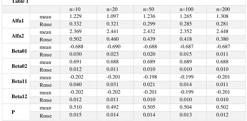
108 indices have been calculated which is presented
in table 1.
As long as the value of RMSE decreases as the sample size increases from
10
, it can beconcluded that that, as the sample size increases the model operates well; as a result, mixture models in the presence of covariates would be a proper fit to the estimate the effects of the covariates in heterogeneous populations.
Table 1
n=10 n=20 n=50 n=100 n=200
Alfa1 mean 1.229 1.097 1.236 1.265 1.308
Rmse 0.332 0.321 0.299 0.285 0.281
Alfa2 mean 2.369 2.441 2.432 2.352 2.448
Rmse 0.502 0.460 0.439 0.418 0.380
Beta01 mean -0.688 -0.690 -0.688 -0.687 -0.687
Rmse 0.030 0.023 0.020 0.015 0.011
Beta02 mean 0.691 0.688 0.689 0.689 0.688
Rmse 0.012 0.011 0.010 0.010 0.010
Beta11 mean -0.202 -0.201 -0.198 -0.199 -0.201
Rmse 0.040 0.031 0.021 0.014 0.011
Beta12 mean -0.202 -0.202 -0.201 -0.199 -0.201
Rmse 0.012 0.011 0.010 0.010 0.010
P mean
0.510 0.492 0.505 0.504 0.502
Rmse 0.015 0.014 0.014 0.013 0.012
Conclusion
In this paper, the Bayesian Weibull mixture model was fitted to the heterogeneous survival data with the help of simulation methods and the proposed model was evaluated by Bayesian estimation methods. In result section, according to the model fitting indices, it was obtained that, this model was a proper fit for the heterogeneous survival data.
References:
1. Kleinbaum D, Klein M. Survival analysis: a self-learning text, Springer Science & Business Media. 2006.
2. Kaplan EL, Meier P. Nonparametric estimation from incomplete observations. Journal of the American statistical association. 1958;53(282):457-81.
3. Cox DR, Snell EJ. A general definition of residuals. Journal of the Royal Statistical Society Series B (Methodological). 1968:248-75.
4. Baghestani A, Moghaddam S, Majd H, Akbari M, Nafissi N, Gohari K. Survival analysis of patients with breast cancer using weibull parametric model. Asian Pac J Cancer Prev. 2015;16(18):8567-71.
5. Erişoğlu Ü, Erişoğlu M, Erol H. Mixture model approach to the analysis of heterogeneous survival time data. Pakistan Journal of Statistics. 2012;28(1):115-30.
6. Erisoglu U, Erisoglu M. L-moments estimations for the mixture of Weibull distributions. Journal of data science. 2014;12:69-85.
7. Berkson J, Gage RP. Survival curve for cancer patients following treatment. Journal of the American Statistical Association. 1952;47(259):501-15.
109 9. Qian J. A Bayesian Weibull survival model:
Duke University; 1994.
10. Marin J, Rodriguez-Bernal M, Wiper M. Using weibull mixture distributions to model heterogeneous survival data. Communications in Statistics-Simulation and Computation. 2005;34(3):673-84.
11. Erişoğlu Ü, Erol H. Modeling heterogeneous survival data using mixture of extended exponential-geometric distributions. Communications in Statistics-Simulation and Computation. 2010;39(10):1939-52.
12. Karakoca A, Erisoglu U, Erisoglu M. A comparison of the parameter estimation methods
for bimodal mixture Weibull distribution with complete data. Journal of Applied Statistics. 2015;42(7):1472-89.
13. Ali S, Aslam M, Ali M. Heterogeneous data analysis using a mixture of Laplace models with conjugate priors. International Journal of Systems Science. 2014;45(12):2619-36.