0 INTRODUCTION
In the laser system for inertial confinement fusion (ICF) [1] and [2], optical devices are essential parts of the power amplifier and the final optics assembly. Defects, such as point defects and line defects on the surface of optical devices, seriously affect the performance of the laser system for ICF. Image processing and pattern recognition technology is widely used for the detection of defects. In [3], laser profilometry is used to detect defects on the surface of power transmission belts. In [4], a defect detection system based on dark-field optical scattering images is designed and assembled for locating and determining the sizes of crystal-originated “particles” (COPs)
on the polished surface of silicon wafers. In [5], a
pulsed eddy current (PEC) thermography system is implemented for notch detection in carbon-fibre reinforced plastic (CFRP) samples and the proposed methods allow the user to observe the eddy current distribution in a structure using infrared imaging and
to detect defects over a relatively wide area. In [6],
a pit-count method based on computer-aided image processing is used for direct measurements of the
cavitation erosion by evaluating the damage on the
surface of the hydrofoil. In [7], methods based on
image processing technology are proposed to detect
the defects on the surface of ceramic tiles. In [8], a
novel visual system is built to recognize erythema migrans. In the visual system, the GrowCut method improved with the new finger draw marker is used to detect potential erythema migrans skin lesion edge, and several methods are used for the classification
of skin lesions into ellipses. In [9], several neural
networks are used for the roughness prediction model of the steel surface machined by face milling. In [10], the regression model and the model based on the application of neural networks are used to predict the machined surface roughness in the face milling of aluminium alloy on a low-power cutting machine.
An apparatus for detecting defects on the surface of optical devices was designed and constructed in the lab of the authors. A high-precision motorized linear stage and a high-precision motorized vertical stage are used to control the line-scan camera moving along the planned path. A series of microscopic dark-field scattering images are collected with the line-scan camera. There is translation transformation
Surface Defect Detection on Optical Devices
Based on Microscopic Dark-Field Scattering Imaging
Yin, Y. – Xu, D. – Zhang, Z. – Bai, M. – Zhang, F. – Tao, X. – Wang, X.
Yingjie Yin – De Xu – Zhengtao Zhang* – Mingran Bai – Feng Zhang – Xian Tao– Xingang Wang
Chinese Academy of Sciences, Institute of Automation, Research Center of Precision Sensing and Control, China
Methods of surface defect detection on optical devices are proposed in this paper. First, a series of microscopic dark-field scattering images were collected with a line-scan camera. Translation transformation between overlaps of adjacent microscopic dark-field scattering images resulted from the line-scan camera’s imaging feature. An image mosaic algorithm based on scale invariance feature transform (SIFT) is proposed to stitch dark-field images collected by the line-scan camera. SIFT feature matching point-pairs were extracted from regions of interest in the adjacent microscopic dark-field scattering images. The best set of SIFT feature matching point-pairs was obtained via a parallel clustering algorithm. The transformation matrix of the two images was calculated by the best matching point-pair set, and then image stitching was completed through transformation matrix. Secondly, a sample threshold segmentation method was used to segment dark-field images that were previously stitched together because the image background was very dark. Finally, four different supervised learning classifiers are used to classify the defect represented by a six-dimensional feature vector by shape (point or line), and the performance of linear discriminant function (LDF) classifier is demonstrated to be the best. The experimental results showed that defects on optical devices could be detected efficiently by the proposed methods.
Keywords: scale invariance feature transform, linear discriminant function, cluster algorithm, image segmentation, image mosaic, dark-field imaging, optical devices
Highlights
• Collected microscopic dark-field scattering images with the line-scan camera.
• Proposed an new image mosaic algorithm based on scale invariance feature transform (SIFT) to stitch dark-field images.
• Proposed a parallel clustering algorithm to obtain the best set of SIFT feature matching point-pairs.
• Used a six-dimensional feature vector to describe the defect.
relationship between the overlaps of adjacent microscopic dark-field scattering images because of the line-scan camera’s imaging feature. In order to obtain the transformation matrix of the overlaps of two adjacent dark-field images, an image mosaic algorithm based on SIFT [11] is proposed. In [12], the simple template matching is used to complete image mosaic. However, the template matching method is not stable and is affected easily by noise. SIFT features are local image features, have higher stability, and are widely used in image registration algorithms
[13] to [15]. Pixel values of defects are much brighter than pixel values of the background in dark-field images, so a sample threshold segmentation method is used to segment images that have been stitched together by the image mosaic algorithm. Defects on the surface of optical devices can be divided into point defects and line defects. In order to effectively identity the types of defects, the performances of four different classifiers (linear discriminant function
(LDF) [16], support vector machine (SVM) [17] to
[19], k-nearest neighbour (KNN) [20] and radial basis
function (RBF) network [21] and [22]) are compared
to select a suitable classifier.
The organization of this paper is as follows. In Section 1, the imaging principle of microscopic dark-field scattering imaging is introduced. The motion path of line-scan camera is also introduced, and the reason for translation transformation relationship between the overlaps of adjacent microscopic dark-field scattering images is explored. In Section 2, the SIFT features is reviewed, and an image mosaic algorithm based on SIFT features is proposed. In Section 3, a sample threshold segmentation method is used to segment images. In Section 4, different classifiers are trained to recognize the types of defects. In Section 5, image stitching experiments and defect classification experiments are carried out, and in Section 6, the ideas discussed throughout the paper are summarized.
1 IMAGING FOR OPTICAL DEVICES’ SURFACE
1.1 Microscopic Dark-Field Scattering Imaging
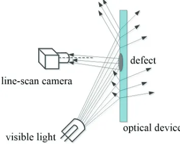
Microscopic dark-field scattering imaging is an ideal means of detecting defects on the surfaces of optical devices. Such surfaces are illuminated by visible light, and some light is scattered by defects on the surface of the optical device. The line-scan camera will receive the scattered light when it collects the images of the surfaces of optical devices, so the defects’ pixel values in the images will be much brighter than the pixel
values of the background (other parts of the optical devices).
Fig. 1. The principle of dark-field scattering imaging
The principle of dark-field scattering imaging is shown in Fig. 1. The geometric-optics model of the
dark-field scattering imaging is analysed in [12], and
a conclusion that the distribution of the light source need to be circular is given.
1.2 Imaging of the Line-Scan Camera
There are two important reasons for using a line-scan camera rather than a plane array camera. First, only one degree of freedom is adjusted to ensure that the line array CCD is parallel to the surface of the optical device when the line-scan camera is used; however, two degrees of freedom need to be adjusted to ensure that the plane array CCD is parallel to the surface of the optical device when the plane array camera is used. Secondly, a high-resolution image (such as Image I1 in Fig. 3) containing all parts of the optical
device in the Z axis direction can be obtained by the
line scan camera; however, if the plane array camera is used, more images need to be taken to contain all
parts of the optical device in the Z axis direction,
and these images need to be stitched to obtain Image
I1. Therefore, the number of images needing to be
stitched is decreased and the running time of the image mosaic is reduced when the line-scan camera is used to acquire the images of the optical devices.
The imaging principle of line-scan camera is shown in Fig. 2. The optical axis of the camera is perpendicular to the surface of optical devices,
and AB is the camera’s field of view, in Fig. 2. The
v Dl f v
m= a, (1)
where vm is the moving speed of the line-scan camera,
D is distance between the camera’s lens and the
surface of optical devices, f is the focal length, l is the pixel size of line-scan camera and va is the line-scan
speed of the line-scan camera.
Fig. 2. The imaging principle of line-scan camera
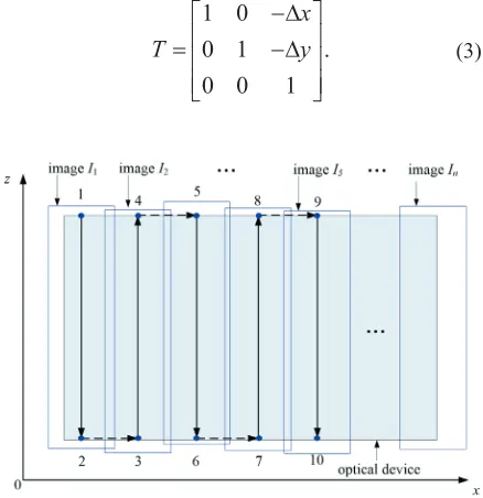
A high-precision motorized linear stage and a high-precision motorized vertical stage are used to
control the line-scan camera moving along the X
axis and Z axis, shown in Fig. 3, and the surface of
optical devices is parallel to the XZ plane. The
line-scan camera is controlled to move from Point 1 to
Point 2 along the opposite direction of the Z axis by
the high-precision motorized vertical stage and dark-field images are collected by the line-scan camera at the same time. Following that, the line-scan camera is controlled to move from Point 2 to Point 3 along
the direction of the X axis by the high-precision
motorized linear stage and the line-scan camera does not collect images in this process. Next, the line-scan camera is controlled to move from Point 3 to Point 4 along the direction of the Z axis by the high-precision motorized vertical stage, and dark-field images are simultaneously collected by the line-scan camera. Next, the line-scan camera is controlled to move
from Point 4 to Point 5 along the direction of the X
axis by the high-precision motorized linear stage, and the line-scan camera does not collect images in this process. The line-scan camera moves according to the above movement rule until the images collected by the camera include the entire surface of the optical device. Finally, dark-field image set I shown in Fig. 3 and Eq. (2) is obtained.
I =
{
I I1, , ,2 In}
. (2)The conclusion that the relationship between the overlaps of adjacent dark-field images such as image I1 and image I2 is the translation transformation
T, shown in Eq. (3), can be easily drawn from the
imaging principle shown in Fig. 2 and the moving path (shown in Fig. 3) of the line-scan camera.
T
x y
=
− −
1 0 0 1
0 0 1
∆
∆ . (3)
Fig. 3. The motion path of the line-scan camera
Δx is the horizontal offset of adjacent
dark-field images’ overlaps and Δy is the vertical offset of adjacent dark-field images’ overlaps. Usually, the
vertical offset Δy is caused by kinematic errors of the high-precision motorized vertical stage, and the
horizontal offset Δx is mainly caused by the setting
value. The horizontal offset Δx usually is set at 300 to 400 pixels in order to balance the number of feature points and the speed of the image mosaic algorithm.
Therefore, the value of Δx is much larger than the
value of Δy (usually the value of Δy is less than 10 pixels).
2 IMAGE MOSAIC BASED ON SIFT
Feature point matching is widely used to stitch images. SIFT features are invariant to image scale and rotation, and are shown to provide robust matching across a substantial range of affine distortion, change in 3D viewpoint, addition of noise, and change in
illumination [11]. An image mosaic algorithm based
The image mosaic principle is shown in Fig. 4. SIFT feature matching point-pairs were extracted from regions of interest in the adjacent dark-field images. The best set of SIFT feature matching point-pairs were obtained by parallel clustering algorithms. The transformation matrix of the two images was calculated by the best matching point-pair set and the adjacent dark-field images were stitched by the transformation matrix.
Fig. 4. The image mosaic principle
2.1 SIFT Feature
SIFT features proposed by D.G. Lowe are widely used in image mosaic, object recognition, robotic mapping and navigation, gesture recognition and video tracking. The following steps are taken to generate SIFT features [11]:
Step 1: Scale-space extrema detection. The scale space of an image is produced from the convolution of a variable-scale Gaussian with an input image. The difference of Gaussian scale-space is computed from the difference of two nearby scales. Maxima and minima of the difference-of-Gaussian images are detected by comparing a pixel to its 26 neighbours in 3×3 regions at current and adjacent scales.
Step 2: Accurate keypoint localization. A 3D quadratic function to the local sample is fitted to determine the interpolated location of the extremum and unstable extrema with low contrast and a low response along edges are simultaneously rejected.
Step 3: Orientation assignment for keypoints. Local image gradient directions are used to assign one
or more directions to each keypoint and the image data is transformed relative to the assigned orientation.
Step 4: Generating SIFT feature vector. At the selected scale in the region around each keypoint, the local image gradients are measured to generate a 128-dimensional vector (SIFT feature vector) for each keypoint.
2.2 Clustering and Screening of Matching Point-Pairs
The Best-Bin-First (BBF) algorithm [23] is used
to find the matching point-pairs set S between the
adjacent dark-field images.
S=
{
1s s, , , , ,2 ks ns}
, (4)and
k k k k k
x k y
s=
{
p p1, 2, ,θ L L,}
. (5)where ks is a feature representation of the kth matching
point-pair, kp1 is the position of the matching point in
dark-field image 1, kp2 is the position of the matching
point in dark-field image 2, kθ is the angle between
the vector kp pk
1 2
and the X axis, kLx is length of the
vector kp pk
1 2
’s component along the X axis, kLy is
length of the vector kp pk
1 2
’s component along the
Y axis.
Fig. 5. The features of matching point-pairs
There are bad matching point-pairs in the
matching point-pairs set S. In order to improve the
accuracy of image mosaic, the best matching
point-pair set Sbest must be selected from the set S. In
Section 1.2, a conclusion that the horizontal offset Δx is much larger than the value of Δy is drawn, so kLx
is much larger than kLy. Bad matching point-pairs are
removed from the set S to obtain the set S′ according
k T
θ θ> . (6)
where θT is an angle threshold. A parallel clustering
algorithm, shown in Fig. 6, is designed to obtain the best matching point-pair set Sbest. In the parallel clustering algorithm, the features kLx and kLy of
the matching point-pair are used for clustering of matching point-pairs. The class owning the most matching point-pairs is reserved for generating the set
Sx in the process of kLx clustering and the class owning
the most matching point-pairs is reserved to generate the set Sy in the process of kLy clustering. The best
matching point-pair set Sbest is the intersection of Sx
and Sy.
Fig. 6. The clustering and screening of matching point-pairs
2.2.1 LxClustering Algorithm
One matching point-pair ms′ (1≤m≤n′) is selected
randomly from the set S′.
′ =
{
′ ′ ′ ′}
S 1s s, , ,2 ns . (7)
Matching point-pairs satisfying the inequality
constraint (Eq. (8)) in the set S′ are to generate the set S′1 as a cluster.
Lx ks L s r
x m x
′
( )
−( )
′ ≤ , (8)where k ranges from 1 to n′, Lx(ms′) is the Lx feature of
the matching point-pair ms′, Lx(ks′) is the Lx feature of
the matching point-pair ks′ and rx is a threshold. Next,
another matching point-pair is selected randomly from the remaining matching point-pairs of the set S′, and
the set S′2 is generated in the same way. The iterative
process above is not stopped until all the matching
point-pairs are clustered. The pseudo-code of Lx
clustering algorithm is shown in Fig. 7.
Fig. 7. Lx clustering algorithm
The Ly clustering algorithm is generated
analogous to the Lx clustering algorithm.
2.2.2 The Best Matching Point-Pair Set
The best matching point-pair set Sbest shown in Fig. 8
is the intersection of Sx obtained with the Lx clustering
algorithm and Sy obtained with the Ly clustering
algorithm.
Fig. 8. The algorithm of obtainingSbest
2.3 Translation Transformation Matrix
∆
∆
x W p p
q
y p p
q i
x i y i
q
i
y i y i q = − +
(
)
= −(
)
= =∑
∑
1 1 2
1 2 1 1 ( ) ( ) ( ) ( ) ,
, (9)
where W1 is the width of the dark-field Image 1 shown
in Fig. 5, q is the number of elements in Sbest, ip1(x)
is the X coordinate of the matching point in image
1, ip2(x) is the X coordinate of the matching point in
Image 2, ip1(y) is the Y coordinate of the matching
point in Image 1 and ip2(y) is the Y coordinate of the
matching point in Image 2.
The coordinates of the pixels in Image 2 are translated by the matrix T to finish the image mosaic.
u v u v T T 1 1 =
T . (10)
where (u, v) is the pixel coordinate in Image 2 and
(uT, vT) is the new pixel coordinate in Image 2.
3 IMAGE SEGMENTATION AND CONTOUR EXTRACTION
A sample threshold segmentation method in Eq. (11) is used to segment images because the pixel values of defects are much brighter than pixel values of the background in dark-field images.
f x y f x y T f x y T s ,
,
, ,
( )
=( )
>( )
≤ 2550 (11)
where f(x,y) is the pixel value in the position (x, y),
fs(x,y) is the new pixel value in position (x, y) after
segmentation and T is the threshold.
The contours of the defects are extracted from the
segmented image by the function cvFindContours() in
Opencv[24].
4 DEFECT CLASSIFICATION
4.1 Feature Vectors of Defects
Supervised learning methods are widely used to infer a prediction function from labelled training data. Given a set of N training examples T={(x1, y1), (x2,
y2), …, (xN, yN)} such that xi is the feature vector of the ith example and yi is its label, a prediction function f : X→Y (X is the input space and Y is the output space) is obtained by supervised learning algorithms.
f x F x y y Y
( ) arg max=
( )
, ,∈ (12)
where F: X×Y→R is a scoring function.
Defects on the surface of optical devices can be divided into line defects (labelled as +1) and point defects (labelled as –1), so supervised learning methods can be used to classify the defects. The six main features of defects shown in Eq. (13) are used to train classifiers.
xi =
(
x x x x x xi1, , , , ,i2 i3 i4 i5 i6)
, (13)where xi1 is the area of the defect, xi2 is the area of
the defect’s envelope rectangle, xi3 is the length of the
defect’s contour, xi4 is the ratio of the length of the
defect’s contour and the area of the defect, xi5 is the
ratio of the defect’s area and the area of the defect’s
envelop rectangle and xi6 is the aspect ratio of the
defect’s envelop rectangle.
By using the proposed six-dimensional feature vector, four different supervised learning classifiers (LDF, SVM, KNN and RBF network) are used. The experimental results in Section 5.3 show that the performance of LDF classifier is better than that of the other classifiers.
4.2 LDF Classifier for Two Classes
The LDF classifier approaches the binary classification problems by assuming that the conditional probability density functions p(x|y=+1) and p(x|y=–1) are both normally distributed with mean and covariance parameters (u+1, M+1) and (u–1, M–1) and the class
co-variances (M+1 and M–1) are identical.
Based on Bayes decision-making theory, the discriminant rule is: assign xi to +1 if g(xi,+1) ≥ g(xi
,-1) and assign xi to –1 if g(xi,-1) > g(xi,+1), where g(xi,y) shown in Eq. (14) is the linear discriminant
function.
g x y f f
f M x f P y M
i y T i y T y , ,
, ln ( ) ,
(
)
= + = − = − − 1 2 1 1 2 12µ 2 µ µ (14)
where P(y) is the prior probability, µˆy is the
within-class sample mean, and the co-variance M is the
weighted average of the co-variances M+1 and M−1.
M n N M n N M = + + + − −
1 1 1 1, (15)
where N is the number of training examples. M+1 and
M−1 are the within-class sample covariance matrix.
n+1 is the number of training samples labelled as +1,
5 EXPERIMENTS
5.1 Experimental Equipment
As shown in Fig. 9, the experimental equipment principally consists of the motion module, the vision module and the PC control module. The motion module consists of the motorized vertical stage, the motorized linear stage and the focus movement axis. The resolution of the motorized vertical stage
and the motorized linear stage is 1 μm. The vision
module consists of the line-scan camera and the light source. The resolution of the line-scan camera is
8192 pixels, the pixel size is 7×7 μm. The line-scan
camera is controlled by the motorized vertical stage and motorized linear stage to move along the path shown in Fig. 3. Via camera calibration, the parameter
D/f = 1.357 is obtained in Eq. (1). The speed of the
line-scan camera along the Z axis is 30 mm/s. The line-scan speed is 3158 frames per second. The distance of the two adjacent images is between (8192–400) pixels and (8192–300) pixels, and we can ensure that the distance is in the above range by setting the moving distance of the line-scan camera along the direction of the X axis.
Fig. 9. Experimental equipment
5.2 Image Mosaic Experiment
The two adjacent dark-field images (each image is 2048×2048 pixels) collected by the line-scan camera are shown in Fig. 10, and the red line in Fig. 10 is the boundary between the two images.
Fig. 10. Two adjacent dark-field images collected by line-scan camera
Fig. 11. Matching point-pairs of two adjacent dark-field images
Fig. 12. The stitching result for the two adjacent dark-field images
Fig. 13. The classification results of Fig. 12
The region R1 (1648, 0, 2048, 2048) is the region
of interest (ROI) in Image 1 (as shown in Fig. 5); (1648, 0) is the coordinate of the ROI’s top left corner in Image 1 and (2048, 2048) is the coordinate of the
ROI’s bottom right corner in Image 1. R2 (0, 0, 400,
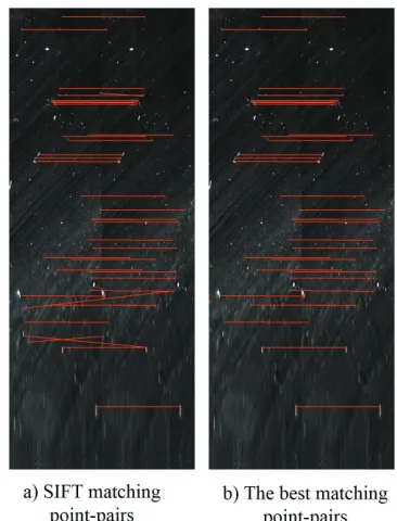
2048) is the ROI in Image 2. SIFT feature points are extracted from the region R1 and R2, and the matching
point-pair set S shown in Fig. 11a is generated by the
(shown in Fig. 11b) is generated by the clustering and screening algorithm introduced in Section 2.2.
In the experiment, θT is set to 10°, rx is set to 20
pixels and ry is set to 20 pixels. The offsets (Δx,Δy)
calculated by Eq. (3) and the set Sbest is (-367,0), so
the matrix T is:
T=
−
1 0 367 0 1 0 0 0 1
. (16)
The stitching result for the two adjacent dark-field images shown in Fig. 10 is shown in Fig. 12 and the red line in Fig. 12 is the boundary between the two images. The results of 15 experiments of image mosaic are shown in Table 1, and the ground truth is obtained by the manual annotation. The maximum
absolute error of Δx is 3 pixels and the maximum
absolute error of Δy is 2 pixels in Table 1.
5.3 Defects Detection and Classification Experiment
A set of 269 training samples including 75 line samples labelled as +1 and 194 point samples labelled as –1 are used to train the four classifiers (LDF, SVM, KNN and RBF network), and a set of 300 testing samples including 86 line samples labelled as +1 and 214 point samples labelled as –1 are used to test the
performance of the four classifiers. The parameter K
of the KNN classifier is set to 1 (a KNN classifier with
the parameter K = 1 also called the nearest neighbour
classifier). The SVM classifier is a Gaussian kernel
SVM classifier with penalty parameter C = 32. The
number of the hidden layers is 50 in the RBF network, and the LDF classifier is trained by Eqs. (14) and (15).
The experimental results of different classifiers are shown in Table 2. The precision of the LDF classifier is higher than the other classifier, so the LDF classifier is more suitable for classifying the defect
represented by a six-dimensional feature vector, shown in Eq. (13).
The classification results of Fig. 12 are shown in Fig. 13. The defects enveloped by red rectangles are labelled as line defects by the LDF classifier and the defects enveloped by blue rectangles are labelled as point defects in Fig. 13.
Table 2. Test Results of different classifiers; test results of the a) LDF classifier, b) SVM classifier, c) KNN classifier, and d) RBF network
Line defects
Point
defects Precision a) LDF
Real quantity 86 214
92.7%
The number of true positives 65 213
The number of false positives 21 1
b) SVM
Real quantity 86 214
86.7%
The number of true positives 63 197
The number of false positives 23 17
c) KNN
Real quantity 86 214
86%
The number of true positives 68 190
The number of false positives 18 24
d) RBF network
Real quantity 86 214
81%
The number of true positives 40 203
The number of false positives 46 11
6 CONCLUSIONS
Methods of defecting defects on the surface of optical devices are proposed in this paper. Translation transformation between the overlaps of adjacent microscopic dark-field scattering images resulted from the imaging feature and the moving path of the line-scan camera. An image mosaic algorithm-based SIFT feature is proposed to stitch the adjacent dark-field images collected by the line-scan camera. A sample
Table 1. Results of 15 experiments of image mosaic
Number 1 2 3 4 5 6 7 8
Ground truth (Δx, Δy) (366, 0) (378, 3) (376, 0) (372, 0) (360, 0) (366, 3) (369, 0) (375, 0)
Measured value (Δx, Δy) (367, 0) (377, 4) (375, 0) (372, 0) (360, 0) (366, 2) (369, 1) (373, 0)
Measurement error of Δx 1 –1 –1 0 0 0 0 –2
Measurement error of Δy 0 1 0 0 0 –1 1 0
Number 9 10 11 12 13 14 15
Ground truth (Δx, Δy) (375, 0) (373, 4) (371, 0) (367, 2) (366, 4) (370, 2) (365, 4)
Measured value (Δx, Δy) (372, 0) (371, 3) (370, 0) (367, 1) (364, 2) (368, 0) (363, 2)
Measurement error of Δx –3 –2 –1 0 –2 –2 –2
threshold segmentation method was used to segment dark-field images according to the characteristic of the stitched dark-field images. The LDF classifier is more suitable for classifying the defect represented by the proposed six-dimensional feature vector. The experimental results showed that defects on optical devices could be efficiently detected by the proposed methods.
7 ACKNOWLEDGMENTS
The paper was supported by National Nature Science Fund of China under Grant 61227804 and 61105036.
8 REFERENCES
[1] Moses, E.I. (2010). The national ignition facility and the national ignition campaign. IEEE Transactions on Plasma Science, vol. 38, no. 4, p. 684-689, DOI:10.1088/0029-5515/53/10/104020.
[2] Cuneo, M.E., Herrman, M.C., Sinars, S.A, et al. (2012). Magnetically driven implosions for inertial confinement fusion at Sandia National Laboratories. IEEE Transactions on Plasma Science, vol. 40, no. 12, p. 3222-3245, DOI:10.1109/ TPS.2012.2223488.
[3] Bračun, D., Perdan, B., Diaci, J. (2011). Surface defect
detection on power transmission belts using laser profilometry.
Strojniški vestnik - Journal of Mechanical Engineering, vol. 57, no. 3, p. 257-266, DOI:10.5545/sv-jme.2010.176.
[4] Lee, W.P., Yow, H.K., Tou, T.Y. (2004). Efficient detection and size determination of crystal originated “particles” (COPs) on silicon wafer surface using optical scattering technique integrated to an atomic force microscope. IEEE Transactions on Semiconductor Manufacturing, vol. 17, no. 3, p. 422-431,
DOI:10.1109/TSM.2004.831531.
[5] Cheng, L., Tian, G.Y. (2011). Surface crack detection for carbon fiber reinforced plastic (CFRP) materials using pulsed eddy current thermography. IEEE Sensors Journal, vol. 11, no. 12, p. 3261-3268, DOI:10.1109/JSEN.2011.2157492.
[6] Dular, M., Širok, B., Stoffel, B. (2005). The influence of the gas content of water and the flow velocity on cavitation erosion aggressiveness. Strojniški vestnik - Journal of Mechanical Engineering, vol. 51, no. 3, p. 132-145.
[7] Rahaman, G.M.A., Hossain, M.M. (2009). Automatic defect detection and classification technique from image: a special case using ceramic tiles. International Journal of Computer Science and Information Security, vol. 1, no. 1, p. 22-30.
[8] Čuk, E., Gams, M., Možek, M., Strle, F., Maraspin Čarman, V., Tasič, J. (2014). Supervised visual system for recognition
of erythema migrans, an early skin manifestation of Lyme Borreliosis. Strojniški vestnik - Journal of Mechanical Engineering, vol. 60, no. 2, p. 115-123, DOI:10.5545/sv-jme.2013.1046.
[9] Saric, T., Simunovic, G., Simunovic, K. (2013). Use of Neural Networks in Prediction and Simulation of Steel Surface Roughness. International Journal of Simulation Modelling, vol. 12, no. 4, p. 225-236, DOI:10.2507/IJSIMM12(4)2.241.
[10] Simunovic G., Simunovic K., Saric T. (2013). Modelling and Simulation of Surface Roughness in Face Milling. International Journal of Simulation Modelling, vol. 12, no. 3, p. 141-153,
DOI:10.2507/IJSIMM12(3)1.219.
[11] Lowe, D.G. (2004). Distinctive image features from scale-invariant keypoints. International Journal of Computer Vision, vol. 60, no. 2, p. 91-110, DOI:10.1023/ B:VISI.0000029664.99615.94.
[12] Yang, Y., Lu, C., Liang, J., Liu, D., Yang, L., Li R. (2007). Microscopic dark-field scattering imaging and digitalization evaluation system of defects on optical devices precision surface. Acta Optical Sinica, vol. 27, no. 6, p. 1031-1038.
[13] Koo, H.I., Cho, N.I. (2011). Feature-based image registration algorithm for image stitching applications on mobile devices.
IEEE Transactions on Consumer Electronics, vol. 57, no. 3, p. 1303-1310, DOI:10.1109/TCE.2011.6018888.
[14] Xu, P., Zhang, L., Yang, K., Yao, H. (2013). Nested-SIFT for efficient image matching and retrieval. IEEE MultiMedia, vol. 20, no. 3, p. 34-46, DOI:10.1109/MMUL.2013.18.
[15] Fan, B., Huo, C., Pan, C., Kong, Q. (2013). Registration of optical and SAR satellite images by exploring the spatial relationship of the improved SIFT. IEEE Geoscience and Remote Sensing Letters, vol. 10, no. 4, p. 657-661,
DOI:10.1109/LGRS.2012.2216500.
[16] Webb, A.R., Copsey, K.D. (2011). Statistical Pattern Recognition. John Wiley & Sons, Hoboken,
DOI:10.1002/9781119952954.
[17] Lim, C., Lee, S.R., Chang, J.H. (2012). Efficient implementation of an SVM-based speech/music classifier by enhancing temporal locality in support vector references. IEEE Transactions on Consumer Electronics, vol. 58, no. 3, p. 898-904, DOI:10.1109/TCE.2012.6311334.
[18] Leiva-Murillo, J.M., Gomez-Chova, L., Camps-Valls, G. (2013). Multitask remote sensing data classification. IEEE Transaction on Geoscience and Remote Sensing, vol. 51, no. 1, p. 151-161, DOI:10.1109/TGRS.2012.2200043.
[19] Qian, H., Mao, Y., Xiang, W., Wang, Z. (2010). Recognition of human activities using SVM multi-class classifier. Pattern Recognition Letters, vol. 31, no. 2, p. 100-111, DOI:10.1016/j. patrec.2009.09.019.
[20] Tan, S. (2006). An effective refinement strategy for KNN text classifier. Expert Systems with Applications, vol. 30, no. 2, p. 290-298, DOI:10.1016/j.eswa.2005.07.019.
[21] Gavrila, D.M. (2000). Pedestrian detection from a moving vehicle. Proceedings of 6th European Conference on Computer Vision, Dublin.
[22] Jayasree, T., Devaraj, D., Sukanesh, R. (2010). Power quality disturbance classification using Hilbert transform and RBF networks. Neurocomputing, vol. 73, no. 7-9, p. 1451-1456,
DOI:10.1016/j.neucom.2009.11.008.
[23] Beis, J., Lowe, D.G. (1997). Shape indexing using approximate nearest-neighbour search in high-dimensional spaces.
Proceedings of IEEE Computer Society Conference on Computer Vision and Pattern Recognition, San Juan,
DOI:10.1109/CVPR.1997.609451.