ISSN: 1942-9703 / © 2013 IIJ
Abstract—This paper discuss the algorithm and real-time implementation of road lane detection and recognition in a miniature vehicle. The research aimed to find an algorithm with low calculation cost intended for real-time implementation in low power and small size embedded system. The algorithm employs probabilistic Hough transform to detect lines and inverse perspective mapping method to recognize the simulated road lane in bird’s view. By using the known distance between lane markings and its color, the algorithm managed to achieve high recognition and vehicle position estimation accuracy. Implementation on an arm-based small processing board yielded a position estimation rate of more than 4 Hz.
Index Terms—Inverse perspective mapping, lane recognition, real-time embedded system, vehicle position estimation.
I. INTRODUCTION
HE position of a vehicle relative to the road lane is one of
the most crucial information for an autonomous vehicle to navigate itself in an urban road environment or in a large factory to automate components and tools deliveries. To be practical, the position estimation must be obtained in real-time and with high accuracy. In some cases such algorithm has to be implemented in a small mobile vehicle, such as in a factory where the vehicle must be small and running on a battery. The computational power is generally limited in such vehicles; hence a low calculation cost algorithm is preferred. Such algorithm can also benefit larger vehicles when less complex lane recognition with minimal cost is required.
Researches on the vision-based lane recognition system have been carried out with various approaches. Most of them are using Hough transform to detect lines in the image [1] [2] [3] [4] [5], however to recognize the lane various methods such as Fuzzy reasoning [6], Gabor filter [7] [8], geometrical model [1] [9], and color features [2] [10] are used. In the process some use the perspective mapping to remove skew caused by the projection of road plane coordinate to the camera coordinate. Some use the warp perspective mapping [7] [4] to estimate the bird’s view of the lane while other use inverse perspective mapping [8]. Many of these approaches specifically handle curved lane [7] [1] [2] [4], while others only handle straight lane.
The authors are with the Computer Engineering Department at Bina Nusantara University, in Jakarta, Indonesia. Sofyan Tan can be reached at: [email protected]. Johannes Mae can be reached at: [email protected].
Many of the approaches however required relatively high calculation cost which is difficult to be implemented in power-limited and small autonomous vehicles. The objectives of this research are to develop a vehicle position estimation system which includes the road lane recognition and the vehicle lateral position estimation algorithms.
For the lane recognition algorithm we use the probabilistic Hough transform [11] integrated in the OpenCV library to speed up line detection. Instead of using the warp perspective mapping, we use the faster inverse perspective mapping [8] to de-skew the lines. However, instead of mapping the image we first perform line detection and only map the line segments to speed up calculation. To improve lane recognition accuracy we also use a priory known color information of the lane markings. The algorithm however only recognize straight lane, assuming that the turning radius is large enough such that the lane in front of the vehicle can be approximated as straight lane up to an adequate distance proportional to the speed of the vehicle.
Furthermore, the algorithm also estimates the lateral position of the vehicle with respect to the center of the lane, and the orientation of the vehicle with respect to the lane direction. We also implemented the algorithm on a small arm-based processing board and evaluated the accuracy of the lane recognition, the lateral vehicle position estimation, and the orientation estimations on a simulated lane.
The following section discusses the line detection implementation, while section III and IV discuss the lane markings recognition in details. Section V discusses the vehicle position estimation based on the recognized lane markings. Section VI explains the experiment setting and the results. Conclusion and future work are presented in Section VII.
II. THE LANE MARKINGS DETECTION
Assuming that the camera’s optical axis is parallel to the flat road lane, the vanishing point of the lane will be at the center row of the captured image. Therefore the information above the center row of the image can be neglected, and further image processing only applies to the lower half of the image to improve calculation speed.
Lane markings are generally designed to have drastic change in brightness at the edges. It is obvious that we can convert the color image into grayscale and use edge detection operator to obtain the edge information in a much smaller
Real-Time Lane Recognition and Position
Estimation for Small Vehicle
Sofyan Tan, Member, IEEE,and Johannes Mae
Computer Engineering Department, Bina Nusantara University, Indonesia
binary edge image.
Since the lane is assumed straight at up to an adequate distance, then most part of the lane markings will show up as straight lines. Lane markings at further distance from the camera will be projected to smaller number of pixels in the image. Hence Hough transform of the edge image will mainly detect lines related to lane markings near to the camera.
Standard Hough transform [12] however takes up a large computational resource since it has to calculate all possible lines passing through all pixels in the image. There has been many researches modifying the standard transform, including the progressive probabilistic Hough transform [11] that we used. This method only transforms some randomly chosen pixels to the parameter space. Furthermore when a group of pixels has been detected to form a line then the rest of the pixels that form the line can be ignored, reducing the calculation time.
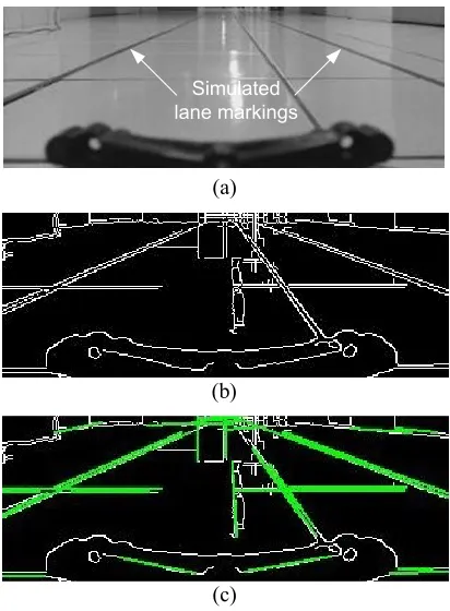
Fig. 1 shows an example of the implemented lane markings detection process, where the lower half of the color image from the camera is converted into grayscale image, and then the Canny edge detection operator is applied to mark edges in the image, and finally the progressive probabilistic Hough transform detect line segments from the edge binary image shown as bold green lines in the Figure. Note that the dark structure at the middle bottom of the image is part of the miniature vehicle protruding into the view of the camera.
Simulated lane markings
(a)
(b)
(c)
Fig. 1. Example of the line detection process, where (a) is the grayscale image, (b) is the edge binary image, and (c) shows the detected lines in bold green.
III. THE INVERSE PERSPECTIVE MAPPING
The current algorithm is optimized to detect solid lane markings. We focus on searching for long solid lines in the
image, omitting short line features with discontinuity. This can eliminate false line detection of irregular shaped structures in the image; however depending on the environment there can be many long straight features other than the lane markings in the image, as in Fig. 1(c). These noises along with the perspective in the image complicate the lane markings recognition in the image plane.
To correct the perspective view of the scene, we can apply perspective mapping methods such as the warp perspective mapping (WPM) and the inverse perspective mapping (IPM). These mappings yields bird’s view estimate of the scene where lane markings are parallel to each other. These methods usually perform mapping of the whole image as in [7] [8].
We can reduce the mapping of the image into the mapping of the line segments using IPM to minimize calculation cost. This only involve mapping of the starting and ending coordinate of each line segment. Assuming the pinhole camera model, we can find the road plane coordinate (X, Z) from the image coordinate (x, y) of each the starting or ending of the line segment according to the following equations
y y
O y
Y F Z
and
x x F
O x Z
X ( ), (1)
where (Ox, Oy) is the image coordinate of the principal point.
Fx and Fy are the focal length of the camera measured in pixels according to the pixel pitch in the column and row direction respectively. The other intrinsic parameters of the camera are assumed to be zero. Note that the intrinsic parameters of the camera can be measured with precision through camera calibration.
The coordinate system of the road plane and the image plane is depicted the Fig. 2. In our case the height of the camera from the road Y is assumed to be constant. The optical axis of the camera is assumed parallel to the lane direction and the optical center is directly above the center of the lane.
X Y
x y
(Ox,Oy) Z
Fig. 2. Coordinate system of the image plane and the road plane where the Z
axis is directly above the center of the lane and parallel to direction of the lane
ISSN: 1942-9703 / © 2013 IIJ However because the extrinsic parameters, which are the
height and orientation of the camera, cannot be kept perfect all the time during operation we expect to see some mapping error. The lane recognition therefore searches for a pair of longest near parallel line segments with distance close to a known value.
Example of the inverse perspective mapping process is depicted in Fig. 3, where line segments detected by the Hough transforms are mapped into the road plane coordinate system. Although there are multiple pairs of near parallel lines, by matching the distance between near parallel line segments we can choose a pair of line segments (in red) that lie at the expected position of the simulated lane markings. Note that there are multiple pairs of line segments that meet the criteria but longer line segments have larger priority to be chosen.
(a)
(b)
Fig. 3. Example of the inverse perspective mapping process, where (a) shows the detected line segments and (b) is the resulting mapped line segments in road plane coordinate (in mm). The red lines are a possible pair of lane markings.
IV. THE COLOR MATCHING
Furthermore, to improve the recognition accuracy by reducing false positive recognition, we add color requirement to qualify a pair of line segments as the recognized lane markings. The color matching process search the pixels in the original color image for a known color feature of the lane markings. This color feature of the lane markings is in HSI (hue-saturation-intensity) color space can be obtained in advance from the actual lane markings as in [2]. The HSI color space divides the color into hue and saturation values. The color information is independent from the illumination
intensity of the image. Therefore we can define some ranges of hue, saturation, and intensity values that fit the known lane markings in various lighting condition.
Initially, the original color image, usually captured in RGB (red-green-blue) color space, is converted to the HSI color space. A binary color mapping is formed by thresholding the original color image according to the chosen ranges of hue, saturation and intensity values. Example of the binary color map is shown in Fig. 4 where the white pixels in the map show the position of the detected dark blue pixels (the color of the lane markings) in the original color image.
Fig. 4. Example of the binary color map of the original color image, showing the position of dark blue pixels.
The color matching process simply searches the binary color map at the position of the candidate pair of line segments and their close surroundings. The candidate pair is the line segments that have meet the previous parallel and distance criteria. Only when the number of dark blue pixels found is above a certain threshold then the candidate pair of line segments is declared as the recognized lane markings.
V. THE VEHICLE POSITION ESTIMATION
If the pair of lane markings are recognized, then we can estimate the lateral error Le of the camera (and therefore the vehicle) from the center of the lane, and the orientation error
θe of the camera’s optical axis with respect to the direction of the lane. Fig. 5 describes the reference frame of the road plane (Xr, Zr) and the camera (Xc, Zc). From the camera frame of reference, the two lane markings have angles θ1 and θ2. The angles are related to the orientation angle error θe from the camera’s frame of reference or to the world angle θw from the road plane’s frame of reference. The Lateral error Le is the distance of the camera from the center of the lane.
Xr Zr
Zc Xc θe
Le θw
θ2 θ1
Fig. 5. The road plane (Xr, Zr) and the camera (Xc, Zc) frames of reference, along with the lateral error Le, orientation angle error θe, first lane angle θ1, and second lane angle θ2.
camera heading deviates toward the right of the lane direction, otherwise the orientation error θe is negative or toward the left of the lane direction. The relation between the lane marking’s angle θn and θe is described in more detail by the following equations.
2 1 2 1 n en e , where (2)
0 when 90 0 when 90 n n n n
en
, n = 1, 2 (3)
The estimated orientation error θe is simply the average of the estimated orientation error from the first lane marking θe1 and from the second lane marking θe2.
Since the distance between the two recognized lane markings is not always equal to the actual lane’s wide, then the lateral error Le is estimated based on the distances of the lane markings to the origin of the camera’s frame of reference. Measurements of the distances are simplified by rotating the lane markings by −θe with respect to the origin of the camera’s frame of reference. The rotation aligns the lane markings to the camera’s Zc axis. Then the distances to the left and right lane markings are simply their abscissa (Xc axis) of the rotated lane marking’s coordinate. The distance from the camera to the lane markings n is calculated according to the following equation
cn cn e e n Y XD cos
sin
, n = 1, 2, (4)where (Xcn, Ycn) is the starting or ending coordinate of a lane marking n. Either the starting or ending coordinate of the lane marking can be closer to the Zc = 0 line. We choose the coordinate (Xcn, Ycn) that is closest to the Zc = 0 line to calculate the distance Dn, because the further the coordinate from the Zc = 0 line, the more it is affected by variation in the extrinsic parameters, and the lesser the accuracy of the inverse perspective mapping.
Note that negative distance means that the lane marking is at the left side of the camera while positive distance is the opposite. The lateral error Le is therefore can be estimated according to the equation
2
2 1 D D
Le . (5)
VI. EXPERIMENT SETTING AND RESULTS
The algorithm is implemented in the Beaglebone board which uses the 720MHz ARM Cortex-8 processor running Linux operating system. Many of the basic image processing functions such as image conversion, Canny edge detection, and progressive probabilistic Hough transform are using the OpenCV library. The camera is the Logitech C920 webcam with a view angle of 78° and the image resolution is set to 320
× 240 pixels. The height of the camera is about 105 mm from the floor. The simulated lane markings used two dark blue adhesive tapes separated at a distance of 48 Cm apart. The tapes are 1 Cm wide and maximum separation distance error is ±5 mm throughout the length of the simulated lane.
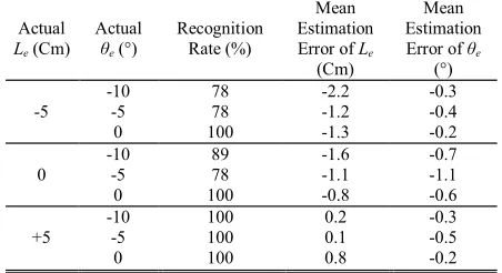
To measure the accuracy of the orientation angle estimation and the lateral error, we put the camera at three different positions with lateral errors: −5 Cm, 0 Cm, and +5 Cm. At each position we evaluate three different orientation error angles of −10°, −5°, and 0°. The camera is positioned manually by hand; therefore we assumed a maximum position error of ±1 mm, and a maximum angle error of ±1° in placement. At each defined position and angle we performed nine trials to recognize the lane and to estimate the lateral and orientation error. The arrangement of the simulated lane and the placement of the camera for evaluation are shown in Fig. 6. 0 Cm +5 Cm -5 Cm 0° -5° -10° 48 Cm
Fig. 6. Placement of the camera for accuracy evaluation.
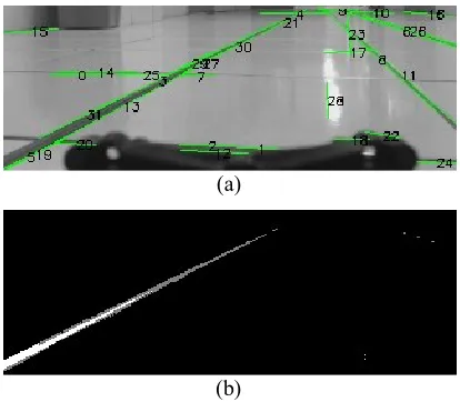
The recognition rate column in Table 1 lists the percentage of successful lane recognitions, each with nine trials. The recognition rate tends to get smaller as the orientation error gets larger. The problem is worse when the lateral error shifts to the same direction as the orientation error. This is because the camera captures less portion of the lane marking at one side as it directs its optical axis to the other side. One example of this condition is shown in Fig. 7 when the lateral error is −5 Cm and the orientation error is −10°. Although line segments are detected at the positions of the right lane markings in Fig. 7(a), however it is difficult to detect the color feature because of the distance Fig. 7(b). Camera with wider view angle will enable lane recognition at larger orientation angle values.
Table 1 also lists the mean estimation error of the lateral error Le. This value is the difference between the mean of the estimated lateral error values and the actual lateral error value.
TABLEI
LATERAL POSITION AND ORIENTATION ERROR ESTIMATION ACCURACY
Actual
Le (Cm) Actual
θe(°)
Recognition Rate (%)
Mean Estimation Error of Le
(Cm)
Mean Estimation Error of θe
(°)
-5
-10 78 -2.2 -0.3
-5 78 -1.2 -0.4
0 100 -1.3 -0.2
0
-10 89 -1.6 -0.7
-5 78 -1.1 -1.1
0 100 -0.8 -0.6
+5 -10 -5 100 100 0.2 0.1 -0.3 -0.5
ISSN: 1942-9703 / © 2013 IIJ Larger estimation error is observed when the camera’s
orientation is heading to the same direction as the lateral error shift. This problem is worst in the sample case in Fig. 7(a). Even when the algorithm manages to detect the right lane marking, the position of the right line segment is less accurate as the distance of from the camera increased. At the other hand, the estimation improves when camera has a close view of the lane markings.
Accuracy of orientation error θe estimation listed in Table 1 is very high, where the estimation error is less than 1 degree in almost all cases.
Evaluation of the calculation speed showed that Beaglebone board can execute the algorithm to calculate 4.2 estimations of the lateral error and orientation error in a second. This calculation rate is adequate in most case for lateral control of the vehicle in normal forward speed.
The most time-consuming calculation in the algorithm is the Hough transformation, which consumes approximately 80% of the calculation time. The authors later found a similar implementation of lane recognition system in [5] using Hough transform and Blackfin 561 DSP processor resulted in a much higher recognition rate. This means that it is possible to significantly improve the calculation speed using the same algorithm with different hardware implementation.
(a)
(b)
Fig. 7. A sample case when (a) the algorithm managed to detect line segments at the far right lane marking position, but (b) unable to detect enough color feature at the far right lane marking.
VII. CONCLUSION
In this research the authors have developed a low-cost algorithm for the recognition of lane markings and the estimation of vehicle’s lateral position and orientation. The image size is cut to half to reduce calculation time. The inverse perspective mapping is performed on the coordinate of detected lines only, not the whole image pixels. The lane recognition rule is very simple, it only searches for two parallel lines with a particular distance to each other. And lastly, to reduce false positive, the color matching step is also very simple, it only checks the color of the pixels around the lane marking candidates.
In general the estimation accuracy of the lateral error and
orientation angle error are highly accurate. Estimation errors of the lateral error are mostly around 1 Cm, this is relatively small if we consider that variation in the lane markings separation and camera placements can reach ±0.6 Cm.
The estimation rate of 4.2Hz is adequate for a small vehicle with a maximum speed of # meter per second. This is calculated based on a conservative assumption that the sensing range is only 2 meter from the camera, and a stopping distance of 0.5 meter. However different implementation in hardware may produce significantly higher estimation rate as demonstrated in [5].
In the future, evaluation using camera with wider view angle is desired to enable higher lane recognition rate in larger orientation angle error. There is still a wide range of possible improvement of the lane recognition algorithm, such as by using the color-thresholded binary image as the input image to speed-up Hough transform. Development and evaluation of a lateral control based on the estimated lateral error and orientation error feedback is also attractive.
A simple proportional lateral control system with low calculation cost should be acceptable for the system since a moving vehicle naturally integrating the lateral error. However the noise of the estimation should be taken care of.
REFERENCES
[1] Shengyan Zhou et al., "A novel lane detection based on geometrical model and Gabor filter," in IEEE Intelligent Vehicle Symposium, San Diego, CA, 2010, pp. 59 - 64.
[2] Ping Kuang, Qinxing Zhu, and Xudong Chen, "A Road Lane Recognition Algorithm Based on Color Features in AGV Vision Systems," in International Conference on Communications, Circuits and Systems, Guilin, 2006, pp. 475 - 479 (Vol. 1).
[3] Shih-Shinh Huang, Chung-Jen Chen, Pei-Yung Hsiao, and Li-Chen Fu, "On-board vision system for lane recognition and front-vehicle detection to enhance driver's awareness," in IEEE International Conference on Robotics and Automation, Taipei, May 2004, pp. 2456 - 2461 Vol.3. [4] Fangfang Xu, Bo Wang, Zhiqiang Zhou, and Zhihui Zheng, "Real-time
lane detection for intelligent vehicles based on monocular vision," in 31st Chinese Control Conference, Hefei, 2012, pp. 7332 - 7337.
[5] Stephen P. Tseng, Yung-Sheng Liao, and Chih-Hsie Yeh, "A DSP-based Lane Recognition Method for the Lane Departure Warning System of Smart Vehicles," in Conference on Networking, Sensing and Control, Okayama, Japan, 2009, pp. 823-828.
[6] Ping Kuang, Qingxin Zhu, and Guochan Liu, "Real-time road lane recognition using fuzzy reasoning for AGV vision system," in
International Conference on Communications, Circuits and Systems, June, 2004, pp. 989-993 Vol.2.
[7] F. Cos kun, O. Tunçer, M.E. Karsligil, and L. Gu venç, "Real time lane detection and tracking system evaluated in a hardware-in-the-loop simulator," in International IEEE Conference on Intelligent Transportation Systems, Funchal, 2010, pp. 1336 - 1343.
[8] A.M. Muad, A. Hussain, S.A. Samad, M.M. Mustaffa, and B.Y. Majlis, "Implementation of Inverse Perspective Mapping Algorithm for the Development of an Automatic Lane Tracking System," in IEEE Region 10 Conference TENCON 2004, 2004, pp. 207 - 210 (Vol. 1 ). [9] A. AM. Assidiq, O. O. Khalifa, Md. Rafiqul Islam, and Sheroz Khan,
"Real Time Lane Detection for Autonomous Vehicles," in International Conference on Computer and Communication Engineering, Kuala Lumpur, 2008, pp. 82-88.
[10] M. Caner Kurtul, "Road Lane and Traffic Sign Detection & Tracking for Autonomous Urban Driving," Bogazici University, Master Thesis 2010. [11] J. Matas, C. Galambos, and J.V. Kittler, "Robust Detection of Lines
and Image Understanding, vol. 78, no. 1, pp. 119-137, April 2000. [12] Richard O. Duda and Peter E. Hart, "Use of the Hough Transformation to
Detect Lines and Curves in Pictures," Communications of the ACM Magazine, vol. 15, no. 1, pp. 11-15, January 1972.
[13] Meng-Yin Fu and Yuan-Shui Huang, "A Survey of Traffic Sign Recognition," in International Conference on Wavelet Analysis and Pattern Recognition, Qingdao, 2010, pp. 119-124.
[14] Ala' Qadi, Steve Goddard, Jiangyang Huang, and Shane Farritor, "Dynamic Speed and Sensor Rate Adjustment for Mobile Robotic Systems," in 19th Euromicro Conference on Real-Time Systems, Pisa, 2007.
Sofyan Tan (M'11) received his B.S. degree in computer
engineering from Universitas Bina Nusantara, Jakarta, Indonesia, in 2002, and his M.Eng. degree in electronic engineering from the University of Tokyo, Tokyo, Japan, in 2008.
He is presently a lecturer at Universitas Bina Nusantara, Jakarta, Indonesia. His research interests include evolutionary computing, visual servoing, embedded systems design, adaptive control systems, wireless channel prediction, and digital wireless modulation.
Johannes Mae was born in Medan, Indonesia. He
received his B.S. degree in computer engineering from Bina Nusantara University, Jakarta, Indonesia in 2012.