SOME PRINCIPLES OF UNSUPERVISED LEARNING AND APPLICATION IN EDUCATION 1

SOME

PRINCIPLES OF

UNSUPERVISED

LEARNING AND

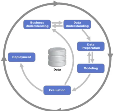
APPLICATION IN EDUCATION

In the beginning of the 90’s the idea of using data stored by computers to inform business really emerged under the name “business intelligence”. Howard Dresner from Gartner has defined business intelligence in 1989 as “concepts and methods to improve business decision making by using fact-based support systems”. Fact-based support systems use data mining to find information hidden in data. The data mining cycle is depicted in Figure Fig. 1.

Fig. 1. Process diagram showing the relationship between the different phases of data mining

source: [4]

Once data have been understood and prepared, which constitutes a substantial amount of work, a number of methods or algorithms can be used for the modelling phase, which is the phase that actually finds patterns. Evaluated patterns give information that can be deployed or used to inform business.

1 _{Published in Varia Informatica 2013, M. Milosz (Ed.), Polish Information}

One distinguishes two categories of methods to discover or learn patterns: the supervised, and the unsupervised methods. The aim of supervised methods is to discover patterns in the data to predict values or labels which are known to exist. For example a bank knows that it has reliable customers who will reimburse their loan, and unreliable customers who will not reimburse their loan. The label reliable / unreliable exists. Supervised methods will be used to try to find the patterns in the data which characterize those customers that are reliable and allows predicting whether a new customer will be reliable or not. The aim of unsupervised methods is to discover labels that are not known in advance. For example a store would like to know whether it has different types of customers, and which ones, to send targeted advertisement. An unsupervised algorithm might discover labels such as „customers who buy mainly expensive dairy products and in-season vegetables” or „customers who buy mainly cheese and wines”.

In this chapter we focus on unsupervised algorithms and present three of them that all belong to clustering: K-means clustering, agglomerative hierarchical clustering and Expectation-Maximisation (EM) clustering2.

Further the idea of business intelligence may well be transferred to education. Thanks to the development of learning managements systems like Moodle and of various tutoring systems, a lot of educational data are available. Why not use data mining on educational data to discover information that might help improve teaching and learning? We complete this chapter by presenting works that use clustering with educational data. The ERAMIS network uses Moodle as a common system. Perhaps students’ projects in learning analytics or educational data mining will be conducted inside the network.

This chapter is organized as follows: first it introduces Euclidean distance in the context of clustering. Then, the three clustering methods mentioned above are presented in turns. Further it is shown, with appropriate data sets, how they differ. Finally, research works applying clustering to data stored by learning systems, in particular Learning Management Systems, are presented. The conclusion summarizes this chapter and gives an outlook. The tool RapidMiner [13] has been used for all examples of this chapter.

1.

Euclidean Distance and Mean

The aim of clustering is to group objects so that similar objects are put in the same group and dissimilar objects in different groups. Some algorithms, like K-means clustering and agglomerative hierarchical clustering, do rely on the fact

2 _{Occasionally clustering is used as a supervised method. We will see such an}

that the similarity or dissimilarity of two objects can be calculated. A distance is a way to calculate how dissimilar two objects are.

The Euclidean distance is well known from school mathematics to calculate the distance between two points in a two-dimensional Euclidean space. Let x

and y be two points with coordinates (x1, x2) and (y1, y2) respectively. Their distance is given by the following formula that can de derived using Pythagoras’ theorem: 2 2 2 2 1 1

)

(

)

(

)

,

(

x

y

x

y

x

y

d

=

−

+

−

In data mining this notion is generalized to any object that can be described by a set of numerical features or attributes. Let us take, as an example, students who are described by their marks in three tests. We assume that the mark of Test 1 is out of 10 points, of Test 2 out of 30 points and of Test 3 out of 50 points. Table 1 shows the marks obtained by three students s1, s2 and s3.

Table 1. Three students and their marks in three tests

Test 1 Test 2 Test 3

s1 8 27 45

s2 9 24 35

s3 7 21 40

Source: own elaboration

Applying the above formula to our students give the following distances:

110

100

9

1

)

35

45

(

)

24

27

(

)

9

8

(

)

,

(

s

=

−

+

−

+

−

=

+

+

=

s

d

In the data mining context, a distance between two objects is always a number bigger or equal to 0. It is equal to 0 when two objects have exactly the same values for the considered set of attributes. In particular the distance between an object o and itself is 0: d(o, o) = 0. The Euclidean distance is sensitive to the order of magnitude of the attributes. Suppose that we scale the three tests above to have them all out of 10 points and that we calculate again the distances between the students. We obtain now the following:

6

4

1

1

)

7

9

(

)

8

9

(

)

9

8

(

)

,

(

s

=

−

+

−

+

−

=

+

+

=

s

d

6

1

4

1

)

8

9

(

)

7

9

(

)

7

8

(

)

,

(

s

=

−

+

−

+

−

=

+

+

=

s

d

With the scaling, the three students are equidistant from each other. Without the scaling, s3 is less distant from s1 than s2.

There are other formulas to calculate the distance between objects and the objects do not have to be described by numerical attributes, see [7]. However, the most common case in business and also in education is to have objects that are described by numerical attributes and the distance used most commonly is the Euclidean distance. We will use Euclidean distance in the sequel.

A group or cluster is often represented by its centre. When Euclidean distance is used, the mean is the most common way to calculate a centre. Using the

mean  the centre of the three students shown in Table 1 is

µ

=

8

+

9

+

7

3

,

27

+

24

+

21

3

,

45

+

35

+

40

3

!

"

#

$

%

&

=

(8, 24, 40).

2.

K-means Clustering

K-means clustering is a partitional clustering method. The number K of desired clusters has to be fixed in advance. We first present the algorithm and then show a method to guess an appropriate K.

Algorithm

K-means clustering discovers or learns clusters by grouping objects of a data set around k centers. It is quite straightforward.

Chose  randomly  K  objects  as  the  initial  cluster  centers  

Repeat  

(Re)assign  each  object  to  the  cluster  which  center  is   nearest  

 Update  the  cluster  means  

Until  no  change.  

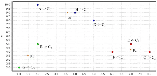
Let us illustrate how the algorithm works with the data set of points shown in Figure 2 when points A, D and G are chosen as initial random centers, which also means that we look for three clusters. Table 2 shows the first two iterations, the first iteration is shown by the three columns on the left and the second iteration by the three columns on the right of the table. Note that for the points A, D and G in the first iteration no calculation needs to be made in the first iteration, because d(o,o) = 0 for any object o. The Euclidean distances are squared because taking the square root has no impact to find the closest center. Further they are left as arithmetic expressions to make their derivation clearer. Consider the distance between B(2, 5) and the center µ1(2, 10) of the first

cluster in the first iteration:

𝑑(𝐵,𝜇!)!=(2−2)!+(5−10)!=(0+25)!, which is written in the table. The values in bold show the smallest distance and, consequently, also the cluster a point belongs to. After the first iteration A is alone in the first cluster, while cluster with center µ3 contains B and G, and the second cluster contains

the remaining points. The attributes of the centers for the next iteration are calculated taking the mean of the points in that cluster, the common way to proceed when Euclidean distance is used as already mentioned. Let us take the third cluster as an example. µ3(x) = (B(x)+G(x))/2=(2+1)/2 = 1.5 and µ3(y)=

(B(y)+G(y))/2=(5+2)/2=3.5, see the new center µ3 in the rightmost column. In

the second iteration H changes from cluster with center µ2 to cluster µ1. A quick

calculation shows that C, D, E and F do not change their cluster in that iteration. In the third iteration, left as an exercise, center µ1 becomes (3, 8.5) and D will

change to this cluster. After that, no change takes place. The final clustering generated with RapidMiner is shown in Figure 3.

Fig. 2. Data set of points from [7] Source: own elaboration

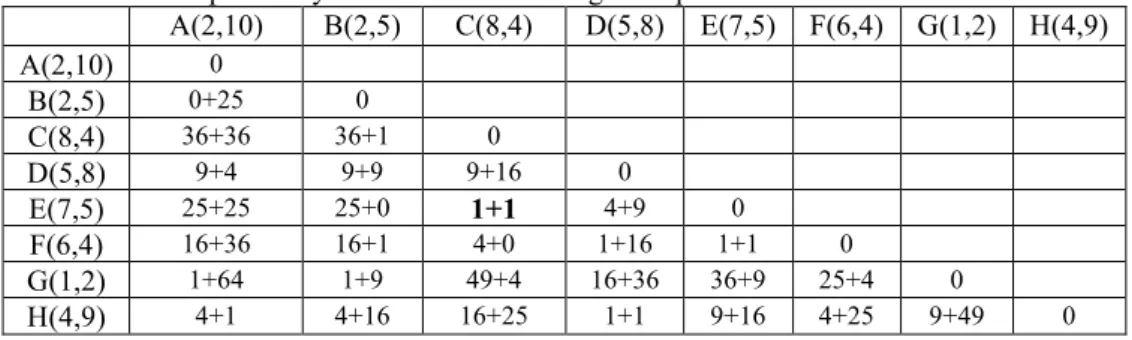
Table 2. The two first iterations to cluster the points of Figure 3 into 3 clusters

First iteration Second iteration

µ1(2,10) µ2 (5,8) µ3 (1,2) µ1 (2,10) µ2 (6,6) µ3 (1.5,3.5) A(2,10) 0 0 B(2,5) 0+25 9+9 1+9 0+25 16+1 0.25+2.25 C(8,4) 36+36 9+16 49+4 36+36 4+4 42.25+0.25 D(5,8) 0 9+4 ₁₊₄ 12.25+20.25 E(7,5) 25+25 4+9 36+9 25+25 1+1 30.25+2.25 F(6,4) 16+36 1+16 25+5 16+36 0+4 20.25+0.25 G(1,2) 0 1+64 25+16 _0.25+2.25 H(4,9) 4+1 1+1 9+49 4+1 4+9 6.25+30.25

Source: own elaboration

A, µ1 D, µ2 G, µ3 B C E F H

Fig. 3. Points of Figure 2 in three clusters Source: own elaboration

Usually clusters are interpreted using their centers. Table 3 shows the centers of the clusters depicted in Figure 3. One can interpret cluster 2 (C2) as

the group of points with large x-coordinate and intermediate y-coordinate, cluster 3 (C3) ,has the points with small x- and y-coordinate, and cluster 1 (C1)

as the points with intermediate x-coordinate and large y-coordinate.

Table 3: Centres of the clusters depicted in Figure 3

Attribute Cluster 1 Cluster 2 Cluster 3

µ(x) 3.67 7.00 1.50

µ(y) 9.00 4.33 3.50

Source: own elaboration

K-means always converges and terminates. This is due to the fact that the sum of squared errors (SSE) diminishes with each iteration. Sum of Squared error is defined as:

∑ ∑

(

µ

In other words, the squared distance between each object and the center of its cluster is calculated and all distances are summed over all clusters. In our example at the end of the first iteration SSE is given by:

d(A, µ1)2 + d(B, µ3)2 + d(C, µ2)2 + d(D, µ2)2 + d(E, µ2)2 + d(F, µ2)2 + d(G, µ3)2 +

d(H, µ2)2 = 67,

where µ1 = (2,1 0), µ2 = (5, 8) and µ3 = (1, 2),

and at the end of the second iteration by:

• µ1 •µ3 •µ2 G -> C3 B -> C3 A -> C1 H -> C₁ D -> C1 F -> C2 E -> C2 C -> C2

d(A, µ1)2 + d(B, µ1)2+ d(C, µ2)2 + d(D, µ2)2 + d(E, µ2)2 + d(F, µ2)2+ d(G, µ3)2 +

d(H, µ1)2 = 30,

where µ1 = (2, 10), µ2 = (6, 6) and µ3 = (1.5, 2.25).

Between any two iterations we observe a drop of the sum of squared errors. Because SSE is a number bigger or equal to 0, at some point the iterations will stop.

It should be noted that the result of K-means clustering, like EM-clustering in the next section, depends on the centers chosen initially. Different centers may give a different result. To overcome this drawback usually K-means is performed several times with several sets of initial centers. The best clustering, the one giving at the end the smallest sum of squared errors, is returned. Further K-means, as EM-clustering, is quite efficient as it contains a simple loop through the data.

Determining the number of clusters

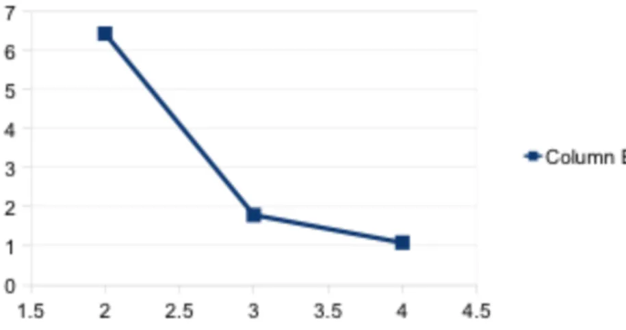
Sometimes users know how many clusters they want to obtain, but most often they don’t. How can we choose K to fit best the data? There are several ways to do so. One way is to use the sum of squared errors again. K-means clustering is performed with several values of K. SSE is plotted against K. If the data do cluster naturally, this plot has an elbow form. The elbow gives the appropriate value for K. Figure 5 shows the plot obtained with K=2, 3 and 4 taking the data set of Figure 3 (note that SSE has been averaged which means divided by the number of objects). In this case 3 is the best choice for K.

Fig. 4. The plot SSE (average) against k shows that 3 is the best number of clusters Source: own elaboration

3.

Expectation Maximization Clustering

Clustering with the Expectation Maximization (EM) Algorithm is similar to K-means clustering, but in contrast to K-K-means distances are not calculated. Instead the probability that an object belongs to a cluster is calculated. The algorithm works with a continuous function –the Gaussian distribution – to calculate the probability of a cluster membership.

The Gaussian distribution

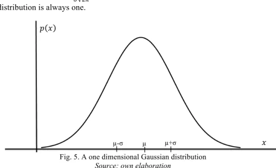
The Gaussian distribution describes the probability of an event. Most phenomena of the nature can be described with this function. It is possible to calculate phenomena that are dependent from many attributes (in that case x, µ and σ would be vectors) but to keep things simple, we are using the Gaussian distribution (figure one) in dependence of only one attribute for our explanation. The probability that x belongs to the Gaussian distribution with arithmetic mean

µ and standard deviation σ is given by:

𝑝 𝑥|𝜇,𝜎 = 1

𝜎 2𝜋𝑒

!  !_!!!!_!!_{=𝒩 𝑥𝜇,𝜎}

where the factor _!!_!! guarantees that the area under the Gaussian distribution is always one.

Fig. 5. A one dimensional Gaussian distribution Source: own elaboration

Data is usually gathered by experiments or observations, in those cases 𝜇 and 𝜎 are unknown, but if there are enough data points they can be estimated by the likelihood method. Let X be a set of N observations assumed to be independent. One looks for a Gaussian distribution with parameters µ and σ, so that the

µ

µ-σ µ+σ

𝑝(𝑥)

probability that each observation can be described by this Gaussian distribution is maximized. Since the observations are independent, the probability that each observation belongs to the Gaussian distribution is the product of the probabilities. So one looks for µ and σ that maximize the following product:

𝐿 𝑋 𝜇,𝜎 = 1

𝜎 2𝜋𝑒

!  !!!!_!!!!

!

!!!

resulting in the following standard estimators:

𝜇= 𝑥! ! !!! 𝑁 and 𝜎 = !!!!   𝑥!−𝜇 ! 𝑁  

EM clustering applies this idea looking for K Gaussian distributions associated to K clusters. The aim of each iteration is to approximate better the K Gaussian distributions of the clusters. In each iteration the probability that the observation or element 𝑥!  belongs to the cluster ck :  𝑝(𝑥!,𝑐!) is calculated.

The calculation is based on the Bayes theorem: 𝑝(𝑥!,𝑐!)=𝑝 𝑐! ∗𝑝 𝑥! 𝑐! ,   𝑤ℎ𝑒𝑟𝑒  𝑐_!  𝑖𝑠  𝑐𝑙𝑢𝑠𝑡𝑒𝑟  𝑘  𝑎𝑛𝑑  𝑥_!  𝑖𝑠  𝑎  𝑑𝑎𝑡𝑎𝑝𝑜𝑖𝑛𝑡   Given  𝑝 𝑥! 𝑐! =  𝒩(𝑥!|𝜇!,𝜎!), we get: 𝑝(𝑥!,𝑐!)=𝑝 𝑐! ∗ 1 𝜎_! 2𝜋𝑒 !  (!!!!)! !!_!!

Maximizing the likelihood of this function gives the following results:

𝑝 𝑐! !"# = 𝑝(𝑥_!,𝑐_!) 𝑁 ! !!! 𝜇_!!"#₌ 𝑝(𝑥!,𝑐!)𝑥! 𝑝(𝑥_!,𝑐_!) ! !!! ! !!! 𝜎_!!"#₌  𝑝(𝑥!,𝑐!) 𝑥!−𝜇!!"# ! 𝑝(𝑥_!,𝑐_!) ! !!! ! !!!

Algorithm

For the EM algorithm, the same routine as in K-means is used: We randomly initialize K µ taking randomly K objects, K is the number of clusters, all σ are initialized with the same random value and  𝑝 𝑐! =1/𝐾. Then we calculate the

probability for each object given a cluster and use that to calculate new µ, 𝑝 𝑐

and σ for each cluster with the given equations. This is done until the centers of the clusters are not changing anymore. The algorithm looks as follows:

Chose  randomly  k  objects  as  the  initial  cluster  centers  

Chose  initial  p(c),  𝜎  for  each  cluster  

Repeat  

  For  each  cluster  

  Calculate  the  probability  that  an  object  belongs  to  

it  

 Update  for  each  cluster  p(c),  𝜇,  𝜎  

Until  no  change.    

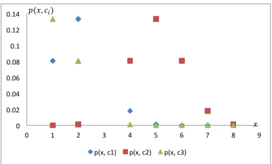
Table 4 gives an example calculation for the first iteration step of EM with the objects shown in Figure 6. The result is shown in Figure 7. One can see that the curves begin to show the typical progression of the Gaussian distribution.

Table 4. Probability that a given datapoint belongs to a cluster after the first iteration. Initial values are: p(c)=1/3,  𝜎 =1  for all clusters and  𝝁𝟏=𝟐,  𝝁𝟐=𝟓,   𝝁𝟑=1   x   p(x,c1)   p(x,c2)   p(x,c3)   2   0,1329 0,0014 0,0806 2   0,1329 0,0014 0,0806 8   2,0252*10-09 0,0014 3,0449*10-12 5   0,0014 0,1329 4,4610*10-05 7   4,955*10-07 _{0,01799 2,0252*10}-09 6   4,4610*10-05 _{0,08065 4,9557*10}-07 1   0,0806 4,4610*10-05 _0,1329 4   0,01799 0,0806 0,0014

Source: own elaboration

Fig. 6. The datapoints Source: own elaboration

Fig. 7. The probabilities that the point belongs to the cluster Source: own elaboration

4.

Agglomerative Hierarchical Clustering

The intuition behind agglomerative hierarchical clustering is to group clusters as long as the resulting groups are too distant. We first present common ways of defining a distance between groups and then the algorithm itself.

Distance between clusters

We present four common and efficient ways to calculate a distance between two clusters or groups of objects. These four definitions rely on using the distance between two objects. We use d both to denote the distance between two clusters and the distance between two objects. Let C1, and C2 be two clusters.

• The minimum distance or single link calculates the distance between

two clusters by taking the minimum of the distances between any two

elements from each cluster:

(

,

)

min

(

,

)

2 , 2 1 2 1 1

o

o

d

C

C

d

=

• The maximum distance or complete link does just the opposite taking

the maximum distance:

(

,

)

max

(

,

)

, 2 1 2 2 1 1

o

o

d

C

C

d

=

• The average distance calculates all distances between any two

elements of each cluster and returns the average or mean distance:

∑

×

=

(

,

)

1

)

,

(

o

o

d

C

C

C

C

d

S

cardinality of a set S.

• The centre distance returns the distance between the centres of the

two clusters:

d

(

C

,

C

)

=

d

(

µ

,

µ

)

µ2 the centre of C2.

Consider the example of Figure 3 and two clusters C1 and C2 with C1 containing

A and H and C2 containing B and G. Applying the four formulas above leads to

the following.

Minimum: d(C1, C2) = min (d(A, B), d(A, G), d(H, B), d(H, G)) = d(H, B).

Maximum: d(C1, C2) = max (d(A, B), d(A, G), d(H, B), d(H, G)) = d(A, G).

Average: d(C1, C2) =

1

2

×

2

Centre: d(C1, C2) = d( (3, 9.5), (1.5, 3.5) ).

Algorithm

Agglomerative hierarchical clustering is rather straightforward too.  

Compute  the  proximity  matrix   Let  each  data  point  be  a  cluster  

Repeat  

 Merge  the  two  closest  clusters    Update  the  proximity  matrix  

Until  only  a  single  cluster  remains.  

Let us illustrate how the algorithm works with our running dataset. The proximity matrix is shown in Table 6. As for K-means we do not take the square root of the distance and leave the expressions. We take the maximum distance or complete link to run the algorithm. There are three pairs of clusters with a squared distance of 2. The first in the alphabetical order, (C) and (E), will be merged as shown in Table 6.

Table 5. The proximity matrix for our running example A(2,10) B(2,5) C(8,4) D(5,8) E(7,5) F(6,4) G(1,2) H(4,9) A(2,10) 0 B(2,5) 0+25 0 C(8,4) 36+36 36+1 0 D(5,8) 9+4 9+9 9+16 0 E(7,5) 25+25 25+0 1+1 4+9 0 F(6,4) 16+36 16+1 4+0 1+16 1+1 0 G(1,2) 1+64 1+9 49+4 16+36 36+9 25+4 0 H(4,9) 4+1 4+16 16+25 1+1 9+16 4+25 9+49 0

Source: own elaboration

The matrix is updated as follows: the distance d(A, (C,E)) is the maximum (d(A,C), d(A,E)) therefore 36+36 in the table. This is repeated for all the remaining objects in the line and column (C,E). Next (D) und (H) will be merged at a squared distance of 2 again, see Table 8. In Table 8 we can see that next (C, E) and (F) will be merged at a squared distance of 4.This continues till all objects are in one cluster.

Table 6. The proximity matrix update after the first merge

A(2,10) B(2,5) C,E D(5,8) F(6,4) G(1,2) H(4,9) A(2,10) 0 B(2,5) 0+25 0 C,E 36+36 25+0 0 D(5,8) 9+4 9+9 9+16 0 F(6,4) 16+36 16+1 4+0 1+16 0 G(1,2) 1+64 1+9 49+4 16+36 25+4 0 H(4,9) 4+1 4+16 16+25 ₁₊₁ 4+25 9+49 0

Source: own elaboration

Table 7. The proximity matrix updated after the second merge A(2,10) B(2,5) C,E D,H F(6,4) G(1,2) A(2,10) 0 B(2,5) 0+25 0 C,E 36+36 25+0 0 D,H 9+4 4+16 16+25 0 F(6,4) 16+36 16+1 ₄₊₀ 4+25 0 G(1,2) 1+64 1+9 49+4 9+49 25+4 0

Source: own elaboration

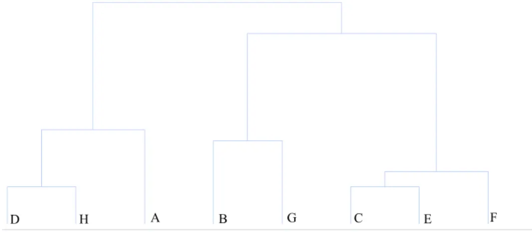
The result of an agglomerative hierarchical clustering is commonly shown as a dendrogram. Fig. 8 shows the dendrogram obtained with our running example. The height of the vertical lines is proportional to the distance while

merging. The dendrogram is cut when the merging distance becomes too big. One notices here that the dendrogram could be cut to yield exactly the same clustering as K-means.

Fig. 8. Dendogram for the points of Figure 2 Source: own elaboration

It should be noted that the result of agglomerative hierarchical clustering depends on the chosen cluster-distance. Further is it less efficient than K-means or EM-clustering as it contains a nested loop through the data. The inner loop comes from updating the similarity matrix.

5.

Comparison and further Issues

With our running example of Figure 2 the three clustering methods give the same result when agglomerative hierarchical clustering is run with complete link. We show, in this section, examples where these methods give different results. Further, we have seen that Euclidean distance is sensitive to the order of magnitude. So are the clustering methods and we illustrate this feature. Finally, can these methods return a clustering even if the data are randomly spread and do not cluster naturally? We finish this section tackling this last issue.

Finding slim shapes

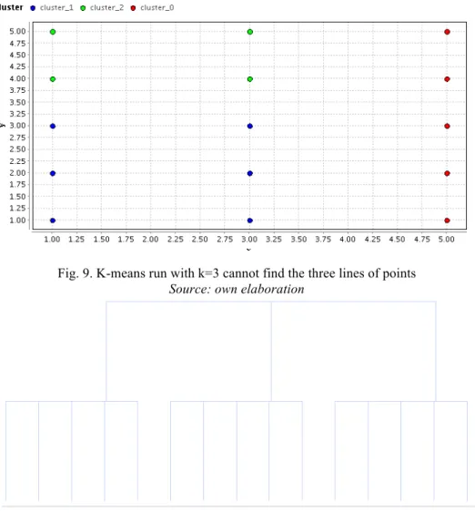
K-means clustering finds round compact shapes with objects distributed around the cluster center. It has difficulties finding slim adjacent groups as Figure 9 shows. Agglomerative hierarchical clustering run with single link can find slim adjacent shapes. The dendrogram Figure 10 is obtained with the dataset of Figure 9. First the three lines of points are found. EM-Clustering cannot find

A

these slim shapes either. It ends with all points in the same cluster but with a very low probability of 0.38 for each point.

Fig. 9. K-means run with k=3 cannot find the three lines of points Source: own elaboration

Fig. 10. Agglomerative hierarchical clustering with single link finds first the three lines of points depicted in Figure 7

Source: own elaboration Scaled data

Numerical attributes can be of different order of magnitude. A distance, such as Euclidean distance is sensitive to the order of magnitude of attributes as we have seen earlier. Therefore, K-means and agglomerative hierarchical clustering, which use a distance, but also EM-clustering are sensitive to the order of magnitude of numerical data as we show now. Consider the two data

sets shown in Table 9. The dataset on the left, used already in the previous section, is the same dataset as the one on the right, except that attribute y uses another unit so that the two attributes x and y have the same order of magnitude.

Table 8. Two datasets: the y-attribute on the right has been scaled down in the dataset on the left x y x y 2 10 2 100 2 5 2 50 8 4 8 40 5 8 5 80 7 5 7 50 6 4 6 40 1 2 1 20

Source: own elaboration

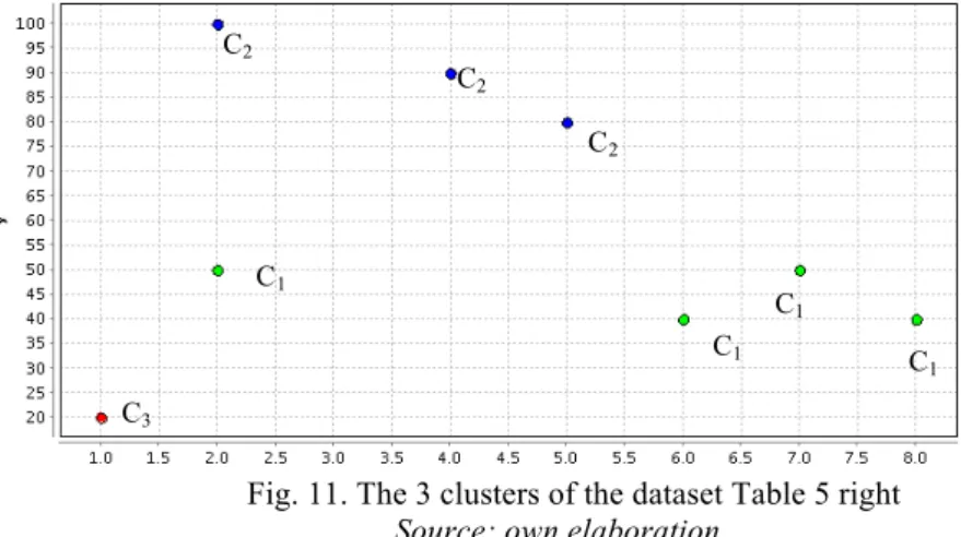
Using the tool RapidMiner, K-means and EM-clustering cluster each of these datasets the same way: exactly in 3 clusters (according to the sum of squared errors, 3 is in both cases the best number of clusters), but the 3 clusters differ: Figure 3 shows the clustering obtained with the dataset on the left, Figure 11 shows it for the dataset on the right. The attribute y with the biggest order of magnitude in the dataset right has more impact on the clustering, and therefore the point (2, 50) belongs to cluster 1 containing points with similar y-coordinates.

Fig. 11. The 3 clusters of the dataset Table 5 right Source: own elaboration

Just looking at the centres does not make any difference. Both clustering methods return centres that are easy to interpret and that can be interpreted in

C1 C1 C1 _C 1 C3 C2 C2 C2

the same way, as can be seen in Tables 10 and 11: Cluster 1 contains points with high x-coordinate and intermediate y-coordinate, Cluster 2 contains points with small x- and y-coordinate, and Cluster3 contains points with intermediate x-coordinate and high y-coordinate.

Table 9. Centers of the clusters Figure 3

Attribute Cluster 1 Cluster 2 Cluster 3

x 7 1.5 3.667

y 4.333 3.5 9

Source: own elaboration

Table 10. Centers of the clusters Figure 11

Attribute Cluster 1 Cluster 2 Cluster 3

x 5.75 1 3.667

y 45 20 90

Source: own elaboration

What is the best clustering? Should the data be transformed so that all attributes have the same order of magnitude, to avoid attributes with bigger order of magnitude to impact primarily the clustering? The answer depends on the context. If the bigger order of magnitude reflects well the bigger importance of the attributes, it might be advisable not to transform the data. Otherwise data should be transformed so that all values have the same order of magnitude. A usual way to proceed is to standardize the data. Weights proportional to their importance can be added to selected attributes.

Random data

Figure 12 addresses the issue of clustering random or uniformly distributed data, though it is not immediately apparent in the figure, as RapidMiner does not use the same scale for the x-axis and the y-axis. Note the difference with Figure 9 earlier, where the points lie on the vertical lines with x-coordinate 1, 3 and 5, and not 1, 2 and 3 as it is the case here. However K-means run with RapidMiner returns 3 clusters when K is set to 3. Simply looking at the centres Table 12, the clusters are easy to interpret: Cluster_0 contains point with intermediate coordinates and small y-coordinates. Cluster_1 contains points with small x-coordinate and big y-coordinate and Cluster_2 contains both points with high x- and y-coordinates. The clusters are interpretable but arbitrary. The sum of square errors helps to find out whether the clustering might be arbitrary: the plot of Figure 4 does not display an elbow form, but a continuous decrease instead. Performing EM-clustering on the same dataset with K set to 3 returns only 1 non-empty cluster with the same low probability for all points (0.469). Probabilities for the two other clusters are lower.

Fig. 12. Arbitrary clusters returned by k_means with radom data Table 11. Centers of the clusters Figure above

Attribute Cluster_0 Cluster_1 Cluster_2

x 2 1.5 3

y 1.5 4 4

Source: own elaboration

6.

Clustering with Educational Data

Education like any other sectors in our society relies more and more on software of different kinds. These software store usage data that can be mined or analysed to understand better how students learn with the goal of improving teaching and learning. This statement is the basis of two emerging fields: educational data mining [5] and learning analytics [9]. Works in those fields use a wide range of techniques to mine and analyse data [2]. Furthermore, a proper visualisation of the results is a crucial aspect in both fields. A common use of supervised techniques is to predict performance: is a student likely to answer an exercise correctly, to pass a course, to drop off a degree? A common use of unsupervised techniques is to find dependencies between attributes and to group objects. They are also combined with supervised or classification methods to obtain better prediction. In this section we give a flavour of how unsupervised methods are used in education by presenting selected works that use clustering.

Some educational software applications, like tutoring systems or serious games, are topic specific. There is a myriad of tutoring systems to learn very specific subjects like algebra middle school, Chinese for beginners, logic proofs

to cite very few examples. The development of a tutoring system requires the help of domain experts and is laborious. The so called intelligent tutoring systems store users' data. Data Mining for this kind of systems consist in analysing usage data and learn from them to adapt to the learner better. For example, an intelligent tutoring system does not propose another exercise on a given topic if the system calculates that the student has already grasped the skills behind, or on the contrary, proposes a similar exercise to reinforce concepts when needed. The calculation of skills' mastery of students is not an easy task. Clustering is combined with classification in [14], [8] and [6] to better calculate skills’ mastery. Clustering is used in [11] to cluster students according to their skills’ mastery: students in one group master or do not master skills in a similar way.

An important class of educational software is the one of Learning Management Systems (LMS) like Moodle. This kind of software is not topic specific, it is at a course level and, to some extend, degree level. LMS make the delivery of contents and the communication between students, teachers and, to some extend, study program managers easier. They store usage data about students' interactions with the contents or resources of a course. Analysing these interactions' data can provide hints and warnings early enough in a course or in a semester about how students are doing. This is especially important for the first semester of any degree where students' drop off is more likely. Analysing these interactions' data provides also valuable hints to improve the resources and the learning and teaching of a course in general, which is a key to students' success.

Pechenizkiy et al. in [12] cluster students according to their results to exercises accessible in a learning management system in order to investigate whether there are groups of students not performing well. They also cluster exercises to investigate whether exercises are related in the following sense: if students fail, respectively succeed, one exercise of a cluster, they also fail, resp. succeed, the others of the same cluster. This can be important to build a well-balanced exam for instance. For this, they use agglomerative hierarchical clustering. They measure the distance between two exercises c and r using conditional probabilities: d(c, r) is the probability of answering c correctly knowing that r has been answered correctly.

Lopez et al. [10] use clustering as a supervised method to predict whether students will pass or fail a course. Interestingly they use only the behaviour of the students in forum for this prediction. They make the assumption that students active in forums will engage more with the material and, consequently, perform better. They get the best results using the following attributes that they calculate for each student: dCentrality: degree centrality, nMessages: number of messages sent, nReplies number of replies sent, nWords: number of words written, dPrestige: degree prestige, aEvaluation: average score of the messages. This means, each object, here a student, is described by six numerical attributes.

The two attributes dCentrality and dPrestige are known from Social Network Analysis. The degree of centrality is usually calculated by the number of messages sent and received, while the degree of prestige is calculated by the number of messages received. The attribute aEvaluation has been manually calculated by a teacher. They have used K-means, EM-clustering and several variants of those algorithms to cluster the students in exactly two groups. One group is expected to be the group of the students who fail the course and the other group the one of the students who pass. They got the best result using EM-clustering with 84% of the students predicted correctly.

The proceedings of the conferences educational data mining (EDM) or learning analytics and knowledge (LAK) present each year works using clustering in an educational setting.

7.

Conclusions

In this chapter we have presented the three most used clustering algorithms, K-means, EM-clustering and agglomerative hierarchical clustering, explaining the ideas they rely on and how they might return different clustering results for the same data sets. We have also presented works that use clustering with educational data.

Inside the ERAMIS network projects in data mining, more specifically in clustering could be conducted. Projects could have to do with the methods themselves: can we visualize how they perform differently on different data sets? Using a tool like RapidMiner it is not possible to see how the centers change with each iteration. A project could be implementing the algorithms in such a way that the centers are visualized after each iteration. Projects could have to do with educational data. In the ERAMIS network the same tests should be given to all students of all partner universities. This will generate data. Can we discover groups of exercises inside a course or even across several courses that students succeed in the same way, as investigated in [12]? Can we discover whether courses are related: students who perform well in course A perform also well in course B? And, of course, projects can be conducted with industrial partners with their own data to support them in improving their business.

8.

Acknowledgements

This work is partially supported by the “Berlin Senatsverwaltung für Wirtschaft, Technologie und Forschung” with funding from the European Social Fund.

References

[1] Baker, R. S. J., Merceron, A., Pavlik, I. J. Jr. (Eds.). Proceedings of the 3rd International Conference on Educational Data Mining, Pittsburgh, USA, 2010 http://www.educationaldatamining.org/EDM2010/

[2] Baker, R. S. J., Yacef, K. 2009. The State of Educational Data Mining in:

A Review and Future Visions. Journal of Educational Data Mining.,

3-17, 2009.

[3] Barnes, T., Desmarais, M., Romero, C., Ventura, S.. Proceedings of the 2nd International Conference on Educational Data Mining. (Cordoba, Spain, July 1-3). EDM’09. 2009

http://www.educationaldatamining.org/EDM2009/

[4] Cross Industry Standard Process for Data Mining http://www.crisp-dm.org/ last accessed April 28, 2013.

[5] Educational Data Mining. http://educationaldatamining.org/ last accessed April 28, 2013.

[6] Feng, M., Heffernan, N., Pardos, Z., Heffernan, C.. Comparison of

Traditional Assessment with Dynamic Testing in a Tutoring System.

International Conference on Educational Data Mining, Eindhoven, Netherlands, 2011, pp. 295–299.

[7] Han, J.W., Kamber, M.. Data Mining: Concepts and Techniques, 2nd edition Morgan Kaufmann. 2006

[8] Gong, Y., Beck, J. E., Hefferman, N. T.. Using multiple Dirichlet

distributions to improve parameter plausibility. In [1], pp. 61-70.

[9] Learning Anayltics. http://www.solaresearch.org/ last accessed April 28, 2013.

[10] Lopez, M. I., Romero, R., Ventura, V., Luna, J.M. Classification via clustering for predicting final marks starting from the student

participation in Forums, Proceedings of the 5th International Conference

on Educational Data Mining,Chania, Greece, 2012, pp. 148-151. [11] Nugent, R., Dean, N., Ayers, E. Skill Set Profile Clustering: The Empty

K-Means Algorithm with Automatic Specification of Starting Cluster

Centers. In [1] pp. 151-160

[12] Pechenizkiy, M., Calders, T., Vasilyeva, E., and De Bra, P. Mining the Student Assessment Data: Lessons Drawn from a Small Scale Case

Study. In [1], pp. 187-191.

[13] RapidMiner. http://rapid-i.com/ last accessed April 28, 2013.

[14] Ritter, S., Harris, T., Nixon, T.,Dickison, D., Murray R. C., Towle, B. 2009. Reducing the Knowledge Tracing Space. In [3], 151-160.

Authors:

Agathe Merceron

Department of Computer Science and Media Beuth University of Applied Sciences Luxemburgerstrasse 10

13353 Berlin, Germany

Ph.D., Responsible of the online degrees Computer Science and Media, Bachelor and Master

Scientific area: Computer Science, educational data mining, learning analytics.

Helena Dierenfeld

Department of Computer Science and Media Beuth University of Applied Sciences Luxemburgerstrasse 10

13353 Berlin, Germany

M.Sc., Research fellow for educational data mining

Scientific area: Computer Science, educational data mining, bioinformatics