SPATIO-TEMPORAL INTEGRAL EQUATION METHODS WITH APPLICATIONS
Dangxing Chen
A dissertation submitted to the faculty at the University of North Carolina at Chapel Hill in partial fulfillment of the requirements for the degree of Doctor of Philosophy in the Department of
Mathematics in the College of Arts and Sciences.
Chapel Hill 2017
Approved by: Jingfang Huang Jianfeng Lu
ABSTRACT
Dangxing Chen: Spatio-temporal Integral Equation Methods with Applications
(Under the direction of Jingfang Huang and Jianfeng Lu)
Electromagnetic interactions are vital in many applications including physics, chemistry, material sciences and so on. Thus, a central problem in physical modeling is the electromagnetic analysis of materials. Here, we consider the numerical solution of the Maxwell equation for the evolution of the electromagnetic field given the charges, and the Newton or Schrödinger equation for the evolution of particles. By combining integral equation techniques with new spectral deferred correction (SDC) algorithms in time and hierarchical methods in space, we develop fast solvers for the calculation of electromagnetism with relaxations of the model in different scenarios.
The dissertation consists of two parts, aiming to resolve the challenges in the temporal and spatial direction, respectively. In the first part, we study a new class of time stepping methods for time-dependent differential equations. The core algorithm uses the pseudo-spectral collocation formulation to discretize the Picard type integral equation reformulation, producing a highly accurate and stable representation, which is then solved via the deferred correction technique. By exploiting the mathematical properties of the formulation and the convergence procedure, we develop some new preconditioning techniques from different perspectives that are accurate, robust, and can be much more efficient than existing methods. As is typical of spectral methods, the solution to the discretization is spectral accurate and the time step-size is optimal, though the cost of solving the system can be high. Thus, the solver is particularly suited to problems where very accurate solutions are sought or large time-step is required, e.g., chaotic systems or long-time simulation.
media Helmholtz equations in the acoustic and electromagnetic scattering problems. With the method of images and integral representations, the spatially heterogeneous translation operators are derived with rigorous error analysis, and the information is then compressed and spread in a fashion similar to fast multipole methods. The preliminary results suggest that our approach can be faster than existing algorithms with several orders of magnitude.
ACKNOWLEDGEMENTS
First and foremost, I would like to thank my thesis advisers, Professor Jingfang Huang and Jianfeng Lu, whose guidance and advice has been indispensable over these past four years. I am especially grateful for the freedom that they have allowed in my research, as well as their unique perspective on computational science and mathematical modeling, which will no doubt shape my own philosophy as I move forward.
I would like to thank my collaborators: Dr. Bo Zhang, Dr. Chao Yang, Dr. Wenzhen Qu, Xingjian Guo. Special thanks are given to Professor Lin Lin for his numerous support and the fruitful work and discussion we had together. Without his help, my achievements would not be possible.
I would also like to thank the tremendous support and encouragement I received from other professors at the University of North Carolina, especially from Professor Katherine Newhall and Professor Jeremy Marzuola.
I am indebted as well to my fellow students (past and present), with whom I have shared this incredible journey. Special thanks go to Yan Feng, Yuan Gao, Wenhua Guan, Feng Shi, Hsuan-Wei Lee, Yanni Lai, Fuhui Fang, Tim Wessler, Jason Pearson, Taoran Li, Xianchao Huang, Yifan Yao, Zhengkan Yang, Meiguo Wang. I would also like to express my deep appreciation to the wonderful staff at the University of North Carolina: Laurie Straube.
TABLE OF CONTENTS
LIST OF FIGURES . . . viii
LIST OF TABLES . . . ix
LIST OF ABBREVIATIONS . . . x
CHAPTER 1: INTRODUCTION . . . 1
1.1 Electromagnetic field . . . 2
1.2 Electronic structure theory . . . 6
1.3 Layered media problem . . . 13
1.4 Outline of the dissertation . . . 18
CHAPTER 2: ADVANCED ITERATIVE METHODS IN TIME . . . 20
2.1 Introduction . . . 20
2.2 Spectral/Krylov deferred correction . . . 23
2.2.1 Collocation formulation . . . 23
2.2.2 Deferred correction . . . 27
2.2.3 Perspective of linear algebra . . . 29
2.2.4 Krylov deferred correction . . . 33
2.3 Convergence analysis . . . 35
2.3.1 Non-stiff systems . . . 36
2.3.2 Stiff systems . . . 37
2.3.3 General cases . . . 39
2.4 Diagonal preconditioners . . . 40
2.5 Optimal preconditioners . . . 47
2.6 Integral equation methods . . . 50
CHAPTER 3: HIERARCHICAL METHODS . . . 61
3.1 Introduction . . . 61
3.2 Fast two-point boundary balue problem solver . . . 63
3.2.1 Integral formulation and tree structure . . . 63
3.2.2 Compression of data . . . 67
3.2.3 Translation of data . . . 68
3.2.4 Algorithm . . . 70
3.2.5 Adaptive algorithm . . . 71
3.2.6 Parallelization . . . 71
3.2.7 Numerical examples . . . 73
3.3 Heterogeneous fast multipole method . . . 73
3.3.1 Spectral representation of the Green’s function . . . 74
3.3.2 Complex image representation . . . 75
3.3.3 Sommerfeld integral representation . . . 76
3.3.4 Compression of data . . . 77
3.3.5 Translation of data . . . 80
3.3.6 Conversion of data . . . 82
3.3.7 Accelerating evaluation of local direct interactions . . . 85
3.3.8 Algorithm . . . 87
3.3.9 Numerical example . . . 91
CHAPTER 4: GENERALIZATIONS AND CONCLUDING REMARKS . . . 93
4.1 More considerations on “optimal" preconditioner . . . 94
4.2 Integral equation method for general cases . . . 94
4.3 Toward a heterogeneous FMM for multi-layered media Helmholtz equations . . . 95
4.4 Conclusion . . . 98
LIST OF FIGURES
1.1 Scattering from a sound-hard obstacle above an impedance plane. . . 16
2.1 Errors of solutions and first integrals for RK4 and Gauss collocation formulation method 27 2.2 Deferred correction for the linear multimode problem . . . 34
2.3 Comparison of deferred correction and Picard iteration . . . 37
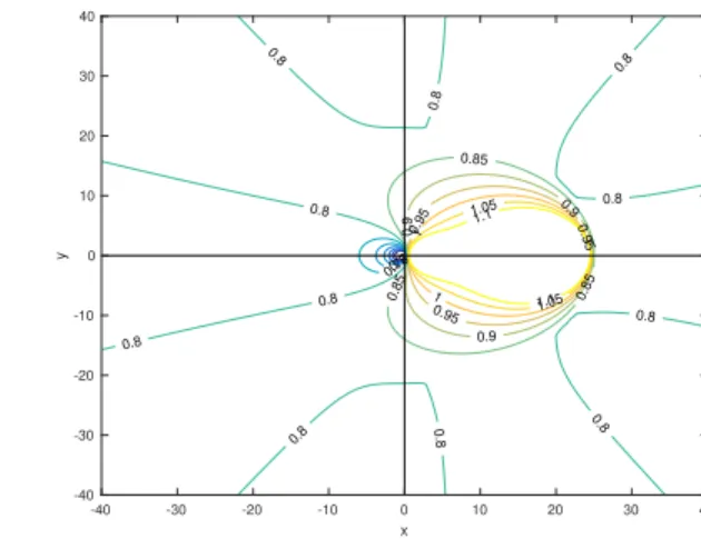
2.4 Contour lines ofρ(C(λ∆t)) form= 5 and m= 10for SDC,λ=x+iy . . . 40
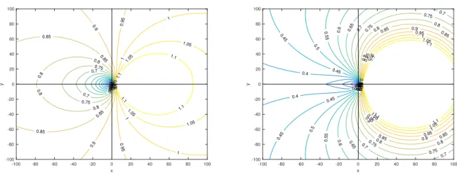
2.5 Contour lines ofρ(C(λ∆t)) form= 5 for triangular (left) and diagonal (right) preconditioners,λ=x+iy . . . 43
2.6 Contour lines ofρ(C(λ∆t)) form= 15for triangular (left) and diagonal (right) preconditioners,λ=x+iy . . . 43
2.7 Contour lines ofρ(C(λ∆t)) form= 5 for triangular (left) and diagonal (right) preconditioners,λ=x+iy . . . 45
2.8 Contour lines ofρ(C(λ∆t)) form= 5 for triangular (left) and diagonal (right) preconditioners,λ=x+iy . . . 45
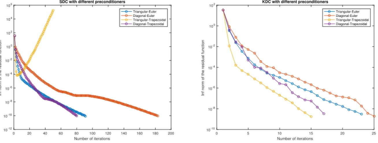
2.9 SDC (left) and KDC (right) for different preconditioners . . . 46
2.10 Contour lines of ρ(C(λ∆t)) form= 10for triangular (left) and “optimal" (right) preconditioners,λ=x+iy . . . 49
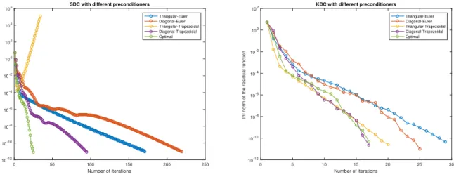
2.11 SDC (left) and KDC (right) for different preconditioners . . . 50
2.12 Comparison for different methods . . . 56
2.13 Conservation laws . . . 56
2.14 Conservation laws . . . 57
3.1 Binary tree for 1-D interval . . . 64
3.2 Yellow box is the target, green boxes are the well-separated boxes . . . 79
3.3 Impedance half-space and notation . . . 80
3.4 Yellow box is the target box; blue boxes along with yellow box is its parent; green boxes are well-separated from them. . . 81
3.5 Yellow box is the source box and the light green is its interaction list. . . 83
3.6 Images are separated to near- and far-field by choosing appropriate C. . . 88
3.7 Uniform distribution in a unit square on top of half-space . . . 92
3.8 CPU time (seconds) for differentN using p= 39andω = 0.1 . . . 92
LIST OF TABLES
2.1 ρ(I−Se−1S) for different numbers of Gauss nodes, stiff case, SDC. . . 38
2.2 ρ(C)of SDC-Lobatto-T, strongly stiff limit case. . . 38
LIST OF ABBREVIATIONS
ADI alternative direction implicit. 21
CFL Courant-Friedrichs-Lewy. 11, 21
DAE differential algebraic equation. 24
ETDRK exponential time-diffencing Runge-Kutta method. 54, 55, 58
FFT fast Fourier transform. 61
FMM fast multipole method. 17, 61, 63, 77, 81, 82, 89–91, 93, 94, 98
GMRES generalized minimal residual method. 17
IEM integral equation method. 19, 22, 23, 54, 55, 57–60 IVP initial value problem. 1, 20, 25, 36, 51
KDC Krylov deferred correction. 12, 22, 23, 33, 35, 41, 44, 49, 62
LDA local density approximation. 10
ODE ordinary differential equation. 11, 12, 18, 20, 21, 23, 25, 35–37, 51
PDE partial differential equation. 11–13, 20, 21, 24, 32, 50, 58, 93
RK4 fourth-order Runge-Kutta method. 27
SDC spectral deferred correction. iii, 12, 18, 19, 21–23, 34, 35, 37, 38, 44, 49, 53, 54, 62, 93, 98
CHAPTER 1 Introduction
The study of material in the presence of external electromagnetic field is central to material science and has provided a rich history of mechanistic insights on interesting phenomenon such as electrostrictive, magnetorestrictive, and piezomagnetic effect, etc. Given a collection of particles in the material, the evolution of the electromagnetic field is determined by the Maxwell equation and the motion of particles are determined by Newton or Schrödinger equation. Given its widespread importance, it is clear that accurate electromagnetic analysis is essential for a faithful physical description of properties of a material, and thus for a quantitative understanding of the response of the material in the presence of electromagnetic field at the classical and quantum level.
In this dissertation, we develop new mathematical and computational techniques for the response of the material under applied fields. Specifically, we discuss the applications of electronic structure theory and layered media problems. electronic structure theory is being used today in an ever-increasing range of applications to widely-varying systems in chemistry, biology, solid-state physics, and material science. Among them, the vast majority of electronic structure calculations today lie in spectroscopy and real-time dynamics in non-perturbative fields [1, 2, 3]. In the simulation, our method relies on a continuum model of the nuclei and electrons with external fields and calculate their motions by solving the Ehrenfest molecular dynamics. The time-dependent Kohn-Sham (TDKS) equation in Ehrenfest dynamics is recast as a Picard type integral equation, which gives it a strong mathematical foundation and then solved using pseudo-spectral collocation formulation by deferred correction method with new preconditioning techniques. In contrast to existing temporal solvers, however, our method is capable of stable arbitrary high-order so that the step-size can be optimal. The result is an iterative solver for the initial value problem (IVP) that is accurate, robust, and symplectic.
[4, 5, 6]. Examples include the design of random media with a well-defined macroscopic refraction (coherent scattering) [5] and the fabrication of metamaterials for cloaking [6], near field imaging and so on. In the calculation, the electromagnetic fields in different layers with external source have to be calculated by solving the Helmholtz equation with complicated boundary conditions. In our method, the Helmholtz equation is reformulated into a second-kind boundary integral equation, which gives it a well-conditioned representation and then solved using a new fast algorithm that can be seen as an example of the hierarchical methods. Different from the existing methods which focus on compressing the integral form of the domain Green’s function, however, our algorithm directly compress the free-space Green’s function and that the information is translated with modified multipole mapping. The result is a solver for the domain Green’s function that is fast, accurate, and robust, with a well-understood mathematical theory and controlled numerical error.
We begin in the next section with a brief introduction of the mathematical formulation of the electromagnetic field, which is a very mature subject [7, 8, 9, 10].
1.1 Electromagnetic field
Consider some moving charged particles in the free space (can be generalized to the case in a matter), what are the fields produced by particles? In the study of electromagnetism in the classical mechanics, the physical laws are governed by the following mathematical equations:
• Gauss’s law: The net electric flux through any closed surface is proportional to the net electric charge within that closed surface. This observation can be formalized as follows:
‹
S
~
E· d~S = 1 0
Q,
where E~ is the electric field, Qis the total charge enclosed within the surface, and0 is the
permitivity of free space. With the help of the divergence theorem and the representation of the charge as integral of the charge density, the equation can be deduced as
˚
V
∇ ·E dV~ = 1 0
˚
V
Since the equation holds for arbitrary closed surface, the differential form can be derived
∇ ·E~ = ρ 0
.
• Gauss’s law for magnetism: The total magnetic flux through a closed surface is zero. Mathematicallly, this implies that
‹
S
~
B·d~S= 0,
whereB~ is the magnetic field. With the help of the divergence theorem, it can be deduced that ˚
V ∇ ·
~
B dV = 0,
from which the differential form is derived
∇ ·B~ = 0.
• Faraday’s Law: A changing magnetic field induces an electric field: the voltage induced in a closed circuit is proportional to the rate of change of the magnetic flux it encloses. This observation can be formalized as follows:
˛
∂Σ
~
E·d~l=− ¨
Σ
∂ ~B ∂t ·d~Σ.
With the help of the Stokes’ theorem, it can be derived that ¨
Σ∇ ×
~
E·d~Σ =− ¨
Σ
∂ ~B ∂t ·d~Σ.
from which the differential form can be derived
∇ ×E~ =−∂ ~B ∂t.
field induced around a closed loop is proportional to the electric current plus rate of change of electric field it enclosed. The observation can be formalized as the following:
˛
∂Σ
~ B·d~l=
¨
Σ
µ0J~+
1 c2
∂ ~E ∂t
!
·d~S,
wherecis the speed of the light andJ~is the electric current. With the help of Stokes’ theorem, it can be deduced that
¨
Σ∇ ×
~ B d~S=
¨
Σ
µ0J~+
1 c2
∂ ~E ∂t
!
·d~S.
Then the differential form can be derived as
∇ ×B~ =µ0J~+
1 c2
∂ ~E ∂t.
Maxwell equation: By the above four laws with mathematical statements, the classical Maxwell equation can be derived as follows:
∇ ·E~ = ρ 0
, (1.1.1)
∇ ·B~ = 0, (1.1.2)
∇ ×E~ −∂ ~B
∂t = 0, (1.1.3)
∇ ×B~ − 1 c2
∂ ~E
∂t =µ0J.~ (1.1.4)
This is the general form of the Maxwell equation, which summarizes the almost entire theoretical content of classical electrodynamics. In the expression, the fields (E~ and B) are put on the left~ whereas the sources (ρand J~) are put on the right to emphasize that all electromagnetic fields are ultimately attributable to charges and currents. What’s more, by applying the divergence to Eq. (1.1.4), the conservation of charge can be derived
∇ ·J~=−∂ρ
The four equations can actually be reduced to two with the introduction of the potential functions. By doing so, the degree of freedom for the electric field is reduced and the generalization to the quantum mechanics is straightforward. From Eq. (1.1.2), the magnetic field can be rewritten as
~
B =∇ ×A.~ (1.1.6)
Then from Eq. (1.1.3), further potential can be introduced such that
~
E=−∇φ−∂ ~A
∂t. (1.1.7)
With the help of potentials, Eqs. (1.1.2) and (1.1.3) are satisfield. Plug Eq. (1.1.7) into (1.1.1), it can be found that
∆φ+ ∂ ∂t
∇ ·A~=−ρ 0
.
Putting Eqs. (1.1.6) and (1.1.7) into Eq. (1.1.4), after some algebra, the equation is arrived as
∇2A~− 1 c2
− ∇
∇ ·A~+ 1 c2
∂φ ∂t
=− 1 c2
0
~ J.
To enforce the invariant of gauge transform
~
A→A~+∇X, φ→φ−∂X
∂t ,
The Coulomb gauge is imposed so that
∇ ·A~ = 0.
gauges such as Lorentz gauge.) Then we end with the coupled equations
∆φ=−ρ 0
, (1.1.8)
∇2A~− 1 c2
−c∇2∂φ∂t =− 1 c2
0
~
J. (1.1.9)
Under the electromagnetic field, the classical particles feel the Lorentz forces
~
F =q(E~ +~v×B),~
where~vis the velocity of the moving charges. Quantum mechanically, particles feels the Hamiltonian operator of the form
H= 1 2
~σ·
−i∇ −1 cA~
2
+φ,
where~σ is the Pauli matrices.
To summarize, Maxwell’s equations tell us how charges produce fields; reciprocally, the force law or Hamiltonian tells us how fields affect charges. In the following sections, we briefly discuss two applications of electromagnetism.
1.2 Electronic structure theory
The electronic structure theory has many applications and plays an important role in quantum chemistry. Consider some atoms consist of nuclei and electrons in the material. Given the applied external electromagnetic field, what are their motions?
In quantum mechanics, the evolution of the state is governed by the Schrödinger equation:
i∂Ψ
∂t =HΨ,
chargeZI in the presence of external fields can be written as
H=
Nnuc
X I=1
P2 I
2MI
+
N X i=1
p2 i
2 +V +Vext.
The physical interpretations of the Hamiltonian are the following:
• PI,pi are the corresponding momemtum operators of the nuclei and electrons
PI =−i∇I, pi=−i∇i.
• V is the interaction potential between the nuclei and electrons
V({R~I},{~ri}) =
1 2
X I6=J
ZIZJ
|R~I−R~J|
+1 2
X i6=j
1 |~ri−~rj|−
X i,I
ZI
|~ri−R~I|
• Vext is the external potential.
Then the Schrödinger equation in this circumstance reads
i∂
∂tΨ({R~I},{~ri}, t) =H({R~I},{~ri}, t)Ψ({R~I},{~ri}, t).
Remark 1.2.1. We want to make some remarks about the model.
• The relativistic effects are neglected in our current formulation. Roughly speaking, the relativistic effects are considered important for heavy atoms, in which the inner electrons are held more tightly to the nucleus and have velocities which approach to the speed of light as the atomic number increase [11, 12].
• For simplicity, the magnetic field is not presented, hence the spin is also neglected. In a diagmagnetic material, all electrons are spin paired and the material does not have a net magnetic field.
with the number of nuclei and electrons. A natural question, therefore, is to ask whether it is possible to treat the nuclei classically. One approach for this is known as the Ehrenfest molecular dynamics [13]. One starts with the separation ansatz for the wave function of the molecular system between the nuclei and electrons [14],
Ψ({R~I},{~ri}, t) = Φ({~ri}, t)X({R~I}, t)ei
´t
0Eee(s) ds,
where
e
Ee(t) = D
Ψ({R~I},{~ri}, t)| He({R~I},{~ri}, t)|Ψ({R~I},{~ri}, t) E
= ¨
Φ∗({~ri}, t)X∗({R~I}, t)HeΦ({~ri}, t)X({R~I}, t) d~r d ~R
and
He({R~I},{~ri}, t) = N X
i=1
p2 i
2 +V({R~I},{~ri}, t) + +Vext({R~I},{~ri}, t).
Taking the inner products with respect toΦ andX and imposing the energy conditions
i
*
X({R~I}, t)|
∂X({R~I}, t)
∂t
+
=DΨ({R~I},{~ri}, t)| H({R~I},{~ri}, t)|Ψ({R~I},{~ri}, t) E
,
i
Φ({~ri}, t)|
∂Φ({~ri}, t)
∂t
=DΨ({R~I},{~ri}, t)| He({R~I},{~ri}, t)|Ψ({R~I},{~ri}, t) E
lead to the so-called time-dependent self-consistent-field equations [15, 16]
i∂
∂tΦ({~ri}, t) =−
X i
∇2 i
2 Φ({~ri}, t) +
D
X({R~I}, t)|V({R~I},{~ri}, t)| X({R~I}, t) E
IΦ({~ri}, t),
i∂
∂tX({R~I}, t) =−
X I
∇2 I
2 X({R~I}, t) +
D
Φ({~ri}, t)| He({R~I},{~ri}, t)|Φ({~ri}, t) E
iX({
~ RI}, t),
of coupled differential equations [16]:
MI
d2
dt2R~I(t) =− D
Φ({~ri}, t)| ∇IHe({R~I},{~ri}, t)|Φ({~ri}, t) E
i, (1.2.1)
id
dtΦ({~ri}, t) =He({R~I},{~ri}, t)Φ({~ri}, t). (1.2.2)
Remark 1.2.2. Ehrenfest dynamics is a potentially powerful technique for modeling atto- to picosecond electron dynamics, but it suffers from the intrinsic problems as its wave function sibling-namely that it is implicitly based on an average potential energy surface and so does not provide state-specific information, and also suffers from problems with microscopic irreversibility.
In Ehrenfest dynamics, Newton’s equation can be solved classically, whereas difficulties still arise in the simulation of Schrödinger equation due to the curse of dimensionality. The Schrödinger equation under the applied field can be written as
i∂
∂tΦ({~ri}, t) =
−
1 2
X i
∇2i +
1 2
X i6=j
1 |~ri−~rj|
+X
i
Vext({~ri}, t)
Φ({~ri}, t). (1.2.3)
Here, one direct external potential from the electronic structure theory is the potential of electron and nuclei
VN e({R~I},{~ri}) =− X
i,I
ZI
|~ri−R~I|
.
For other examples, in many experiments, the laser field is applied
Vlaser({~ri}, t) =Ef(t) sin(ωt) N X
i=1
~ri·~α,
therefore to achieve the dimensional reduction. The density function is obtained with the help of the fictitious system of non-interacting electrons, the Kohn-Sham system. The electrons feel an effective potential, the TDKS potential. The exact form of this potential is unknown and is extremely difficult to derive, and the approximation has to be made. As a consequence, the TDKS equation is of the form
i∂
∂tψj(~r, t) =
−12∇2+VKS(~r, ρ, t)
ψj(~r, t) (1.2.4)
=
−1 2∇
2+V
Hartree(ρ) +Vxc(ρ) +Vext(~r, t)
ψj(~r, t)
where {ψj}are the Kohn-Sham orbitals, VKS is the Kohn-Sham potentials including the Hartree
term
VHartree(ρ) =
˚
V
ρ(~r, t) |~r−~r0| d~r
0
andVxcis the exchange-correlation potential, which must be approximated. One simple choice is
adiabatic local density approximation (LDA), which can be written as
Vext(ρ) =Cρ4/3(~r, t).
The density function is calculated by
ρ=
N X j=1
|ψj|2.
Remark 1.2.3. We want to make some remarks about the model.
• The choice of exchange-correlation potential significantly affects the performance of the TDDFT. However, in the perspective of mathematics, analysis of LDA already give us much information. • In the simulation, the pseudopotential [25, 26] is usually employed to replace the complicated
this term also becomes non-stiff in the language of numerical analysis.
In TDKS equation, challenges arise for the long-time calculation. For example, in the calculations of 5TBA monolayer thin film [27], the final time is around 1 picosecond, whereas the time-step is around attosecond. In such calculations, it is difficult to obtain an accurate solution, and in addition, with well-preserved conservation laws.
The TDKS equation can be solved in many ways, perhaps the simplest of which is via explicit Runge-Kutta methods, which judiciously uses the information on the “slope" at more than one point to extrapolate the solution to the future time step. A mature package with explicit Runge-Kutta methods is well developed in [28].
Another approach is to use low-order implicit methods, such as Crank-Nicolson and Magnus expansions. One particular advantage of them over explicit methods is their stability, which allows for larger time-steps in stiff systems. In numerical analysis language, the Courant-Friedrichs-Lewy (CFL) condition is much relaxed. Progress on low-order implicit methods for the TDKS equation can be found in Octopus (http://octopus-code.org/wiki/Manual), NWCHEM (http://www.nwchem-sw.org/index.php/Main_Page), GPAW (https://wiki.fysik.dtu.dk/gpaw/) as well as other TDDFT software packages.
Splitting type algorithm is also commonly used in the community. The main reason for splitting methods over others is its support for preservation of conservation laws. Discussions of this type can be found in [29, 30].
tool". Since the time is only one-dimensional and there is no complex geometry involved, a natural question is to ask to what extend spectral (pseudo-spectral) methods can be likewise applied.
We consider the pseudo-spectral collocation formulation based on the Picard integral equation. There has been extensively study of this representation for ODEs [35, 36, 37]. The new representation brings with it several favorable qualities, which can be roughly summarized as follows:
• The system is well-conditioned.
• The error of the solution decays rapidly due to the spectral discretization; • The stability of the formulation is usually not an issue;
• The global errors grow slowly;
• The quadratic first integrals are preserved while applying to the conserved system.
The pseudo-spectral collocation formulation is generally considered the optimal formulation since it has a strong mathematical foundation, and is commonly used in second-order parabolic PDEs. This implementation, however, comes at a significant expense, as the discretization by spectral methods leading to a dense system. For aN-dimensional ODE system, ifm nodes are used in time, the overall size of the discretization ismN, and the computational complexity is proportional to (mN)3 if Gaussian elimination is applied, which is prohibited in the large-scale calculation.
recognized as applying the Newton-Krylov method to the preconditioned error equation, effectively eliminate the order reduction.
In this dissertation, we describe several new preconditioning techniques and integral equation formulations in the temporal direction that is quite general. For stiff PDEs, e.g., the TDKS equation, our algorithm is capable of optimal time step-size.
1.3 Layered media problem
In many experiments, the materials are designed by incorporating large numbers of identical inclusions (particles) in a layered material. Given an incoming source electromagnetic field, what is the scattered electromagnetic field?
Since charge and current are absent in the space and therefore, the Maxwell equation reads
∇ ·E~ = 0, (1.3.1)
∇ ×E~ =−∂ ~B
∂t, (1.3.2)
∇ ·B~ = 0, (1.3.3)
∇ ×B~ = 1 c2
∂ ~E
∂t. (1.3.4)
They constitute a set of coupled, first-order, PDEs forE~ andB. Applying the curl to the Eq. (1.3.2),~
(∇ ·E)~ − ∇2E~ =−∂
∂t(∇ ×B).~
With the help of Eqs. (1.3.1) and (1.3.4), it can be derived that
∇2E~ = 1
c2
∂2E~
∂t2 .
In much of same way, applying the curl to Eq. (1.3.4),
∇(∇ ·B)~ − ∇2B~ = 1
c2
∂
With the help of Eqs. (1.3.3) and (1.3.2), it can be derived that
∇2B~ = 1
c2
∂2B~
∂t2 .
Now separate equations forE~ and B~ are obtained. In vacuum, then, each Cartesian component of ~
E and B~ satisfies the three-dimensional wave equation,
∇2f = 1
v2
∂2f
∂t2.
As discussed in [45], a dielectric medium that is linear, isotropic, homogeneous, and nondispersive, all components of the electric and magnetic field behave identically and their behaviors are fully described by a single scalar wave equation. We then turn away from the vector theory to the simple scalar theory. By separation of variables, the wave equation can be simplified. Assume that
f(~x, t) =A(~x)T(t).
Substitute this into the wave equation, we obtain
∇2A
A =
1 v2T
d2T
dt .
This equation is valid only when both sides are constant. By assuming the constant be −ω2 without
loss of generality, we have
∇2A
A =−ω
2,
1 c2T
d2T
dt2 =−ω 2.
Rearranging the first equation, the Helmholtz equation is obtained
Likewise, letk=ωv, the second equation becomes
d2
dt2 +k 2
T = 0.
The solution in time will be a linear combination of sine/cosine functions and the solution in space will depend on the boundary conditions. Hence, by appropriate assumptions, the wave equation can be simplified to the Helmholtz equation. In layered media problems, complicate boundary conditions in each layer are imposed.
Three commonly used methods to approximate the Helmholtz equation in a media are finite difference methods [46], finite element methods [47], and boundary integral methods [48]. In the finite difference method, the region of interest is discretized by a set of points at which the differential operator is approximated by Taylor expansion. For a typical finite element method, the differential equation is recast as a weak formulation, and the computational domain is partitioned into a finite number of small elements in which low-order polynomials approximations are used.
Despite their prevalence, both finite difference and finite elements have the major drawback that when applying to the infinite domain, the entire volume must be discretized with artificial truncation [49, 50]. In contrast, integral equations in this circumstance often require unknown only on the domain boundary, leading to a dimensional reduction in the linear system to be solved. In this sense, integral equation reveals the true size of a problem. This is one of the reasons that we have adopted an integral equation approach. Furthermore, the discretization of the integral equation formulation leads to a well-conditioned linear system. Specifically, the condition number of the corresponding matrix A typically is a constant, which enables more stable convergence. On the other hand, the condition number of finite difference and finite element methods grow as O( 1
h2), where h is the minimum mesh width.
For a review of recent developments in numerical methods for the Helmholtz equation, including finite difference, finite element, and integral equation methods, see [51].
We now turn to a brief treatment of integral equations of Helmholtz equation, using two-layered media problem as an example. For a complete account, including potential and Fredholm theory, we refer the interested reader to [52, 53, 54].
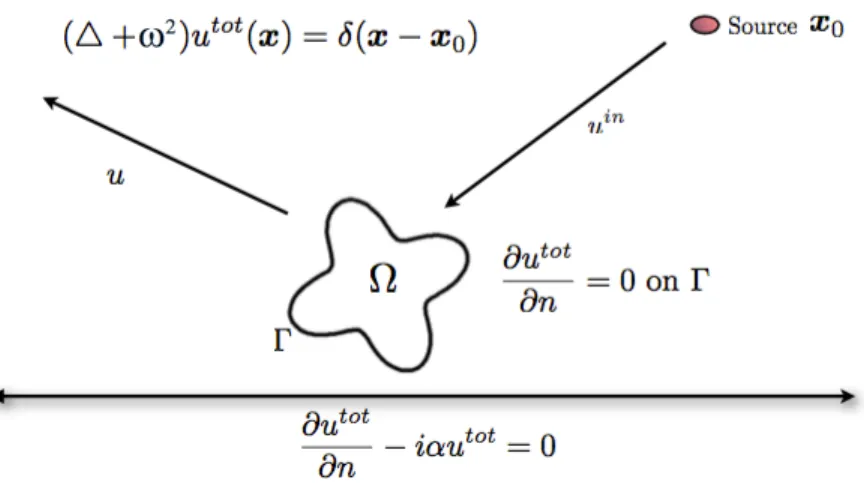
point source located at ~x0 = (x0, y0) in the presence of a “sound-hard" obstacle over an infinite
half-space subject to impedance boundary conditions in Figure 1.3. Let the total field be defined as utot =uin+u, where uin denotes the (known) incoming field due to the point source and udenotes
the scattered field. Since the scattered field involves no sources outside the obstacle Ω, it must satisfy the homogeneous Helmholtz equation
(∆ +ω2)u(~x) = 0.
On the obstacle boundaryΓ, the total field must satisfy homogeneous Neumann boundary conditions
∂u ∂n =−
∂uin
∂n ,
where ∂n∂ is the outward normal derivative. Finally, on the interface, an impedance condition is imposed such that
∂utot
∂n −iαu
tot= 0.
By integral equation methods, an ansatz is to represent the total field as
utot(~x) = ˆ
Γ
gω,α(~x, ~y)σ(~y) d~y+uin(~x),
wheregω,α is the domain Green’s function, i.e., the Green’s function of half-space with homogeneous
impedance boundary conditions, and uin(~x) = g
ω,α(~x, ~x0). Imposing the Neumann boundary
condition on the obstacle yields that Fredholm integral equation of the second kind:
−1
2σ(~x) + ˆ
Γ
∂ ∂nx
gω,α(~x, ~y)σ(~y) d~y=−
∂ ∂nx
gω,α(~x, ~x0)
open that how to evaluate the domain Green’s function efficiently. The domain Green’s function is so complicated that the integral form is usually used to represent it. Satisfying the Sommerfeld radiation condition
lim
r→∞
√ r
∂
∂rgω,α−iωgω,α
= 0
the domain Green’s function can be written in the Sommerfeld representation
gω,α(~x) =
1 4π
ˆ ∞
−∞
e−√λ2−ω2(y+y 0) √
λ2−ω2 e
iλ(x−x0) √
λ2−ω2+iα
√
λ2−ω2−iα !
dλ
or in the form of
gω,α(~x) =gk(~x, ~x0−2y0by) + 2iα
ˆ ∞
0
gk(~x, ~x0−(2y0+η)y)eb iαη dη
with the help of method of images. Here, ~x0 = (x0, y0) is the location of the source, gk is the
free-space Green’s function, and by= (0,1).
The main contribution previously along this direction has been focusing on compress the discretization of the integral form of the domain Green’s function [58, 59, 60, 61, 62, 63, 64, 65, 66]. Unfortunately, this approach is considered inefficient as the data is too complicated to compress. In this dissertation, the free-space Green’s function is compressed, the modified translation formulas are derived, and then the information is translated in the hierarchical tree structure in the fast multipole fashion. One striking feature of our method is its efficiency: the computational complexity is similar to the evaluation of Green’s function in free space and the algorithm can be orders of magnitude faster than existing schemes for simulating 2-D waves in two-layered media.
1.4 Outline of the dissertation
The remainder of this dissertation is organized as follows.
In Chapter 3, we discuss applications of the hierarchical methods. We begin with the parallel version of the fast hierarchical solver for two-point boundary value problem, which has been used as a preconditioner for SDC. Then we introduce a new hierarchical method for layered media problem. This is followed by complexity and error analysis, which we verify through extensive numerical experiments.
CHAPTER 2
Advanced Iterative Methods in Time 1
2.1 Introduction
The construction of efficient, stable, and high-order methods for solving the IVP is, in many respects, a mature subject. For ODE IVPs, the linear multistep methods and Runge-Kutta methods have been extensively studied in both theory and implementation [67, 68, 69, 70]. Widely used ODE IVP solvers include the backward differentiation formula based DASPK [71, 72] and Runge-Kutta method based Radau5 [73]. We refer interested readers to [74] for existing theoretical results, different algorithms, and software packages. Many of these numerical simulation tools have been successfully applied in research studies and have significantly advanced our knowledge in science and engineering. However, these advances in turn also revealed the limitations of existing numerical algorithms, which can be roughly divided into two classes of systems:
• chaotic system: one example is the simulation of Kuramoto-Sivashinsky equation [75, 76], which models thermal diffusive instabilities in laminar flame fronts. The solution of PDE can exhibit chaotic behaviors. For instance, the perturbation of initial data can be amplified by as much as 108 up to time t = 150. Given the lack of confidence of existing methods, it is
important to obtain a very accurate result to study and explore the chaotic solutions in the systems. However, the generalization of the existing methods from low-order to higher-order, especially in stiff systems, is not straightforward.
• long-time dynamic: for instance, difficulties arise in the simulations of electron dynamics with applications in the electronic structure theory by real-time time-dependent density functional
1
theory [18, 77, 1, 2]. In this simulation, scientists are interested in the phenomena occurred in the scale of picosecond (10−12 second) or even longer, whereas the time scale of the system is
attosecond (10−18second). There are several difficulties in simulating such long-time dynamics
using the existing algorithm, including the stability restriction (CFL condition) and accuracy restriction (due to low-order) of the step-size, as well as the fast growth rate of the global error. Our primary goal is to improve the performance of the algorithm in these regards.
In this chapter, we study a new class of time-stepping method by (pseudo-) spectral methods. We begin by converting the original ODE into the corresponding Picard equation, which has several analytical advantages. However, the discretization leads to a large dense matrix. The standard direct method, such as Gaussian elimination will be computationally intractable in the large-scale calculation. To efficiently solve the system, iterative methods such as deferred correction are proposed. The resulting SDC has been successfully applied to many problems and have shown advantages in the high-accuracy regime. Unfortunately, when applying to the stiff system, the performance of the deferred correction methods deteriorate and order reduction is observed. Several approaches are proposed to improve the performance of the deferred correction scheme, which can be classified, loosely speaking, into three groups.
• Low-order methods: the first group seeks different low-order preconditioners to have a better-conditioned system or to reduce the computational complexity. In [40], higher-order precondi-tioners based on Runge-Kutta with uniform grids are proposed and analysis indicates that preconditioners with uniform sampling have better performance; in [78], operator splitting methods are served as the preconditioner and show some advantages; in [42], the alternative direction implicit (ADI) approach is used as a preconditioner in parabolic PDEs with lin-ear complexity; in [79], multigrid methods are used in the temporal direction to reduce the computational cost.
examples [83].
• Krylov subspace methods: by re-formulating the SDC in the framework of linear algebra, the deferred correction approach can be recognized as applying the fixed-point iteration to a preconditioned error equation. In particular, for linear problems, the deferred correction is equivalent to a Neumann series, which motivates researchers to use the Krylov subspace method to accelerate the convergence. The resulting KDC [43, 44] effectively eliminate the order reduction with more memory usage and some overhead calculations.
In this dissertation, we develop new mathematical and computational techniques for the accurate and efficient solutions by collocation schemes. First, motivated by the success of parareal idea in the temporal direction, we introduce a new class of diagonal preconditioner. Different from the parareal SDC, which performed over multiple time-steps in parallel, the diagonal preconditioner aim to parallelize the function evaluation in every single local interval. Furthermore, our analysis indicates that the diagonal preconditioner is more stable than the traditional triangular preconditioner. Preliminary results suggest that the diagonal preconditioner is capable of achieving high parallel efficiency and show some advantages in the modern computer architecture.
Secondly, we have noticed there exist many powerful low-order preconditioners and each of them has certain advantages and disadvantages. A natural question is to ask how to choose a preconditioner with optimal performance under certain conditions. To improve the performance of the deferred correction, we propose a preconditioning technique, which combines different preconditioners, to train an “optimal" preconditioner to optimize the conditioning of the preconditioned system. The optimization procedure can be calculated in the precomputation stage. As a result, the iteration number by deferred correction with “optimal" preconditioner is reduced significantly.
The chapter is organized as follows. Section 2.2 briefly reviews the spectral and Krylov deferred correction. The performance of the deferred correction is analyzed in Section 2.3. Our new precon-ditioning techniques diagonal preconditioners, “optimal" preconditioners, and IEM are introduced in Section 2.4, 2.5, and 2.6, respectively. Finally, in Section 2.7, the application to the TDDFT is discussed. Materials in the Section 2.3 has been presented in [84] and papers reporting on Section 2.4-2.6 is in preparation [85, 86].
2.2 Spectral/Krylov deferred correction
In this section, we briefly review the SDC [38] and KDC [43]. We begin by discussing the collocation formulation of the differential equation with rigorous analysis. Then the deferred correction scheme is described to solve the system. The perspective from linear algebra is provided for better understanding of the algorithm. Finally, we discuss how the Krylov subspace methods can be used to accelerate the convergence of the deferred correction.
2.2.1 Collocation formulation
For simplicty, consider the 1-dimensional ODE of the form
y0(t) =f(t, y), t∈[0, T],
y(0) =y0
(2.2.1)
wherey and f are assumed to be smooth, which is the requirement for high-order construction. In addition, we focus on the single interval with refinementt0, t1, . . . , tm, tm+1 such that
t0= 0, tm+1=T,
t0≤t1< t2 <· · ·< tm ≤tm+1.
We use Gauss-Legendre points t1, . . . , tm in time, unless otherwise stated. We also denote∆tas the
length of the interval[0, T]and∆tn astn+1−tn.
is recast as a Picard integral equation,
y(t) =y0+
ˆ t
0
f(τ, y) dτ.
The integral equation formulation gives us a well-conditioned system as the numerical integration is more stable than numerical differentiation.
Remark 2.2.1. The maximum of spectral differentiation grows like O(m2), whereas the maximum
eigenvalue of spectral integration matrix is bounded, and the minimum eigenvalue decays likeO( 1 m2).
For discretization, first we consider the y-formulation. Sincef smooth, given the values ofy,e we interpolate it with a high-order orthonormal polynomial. In Lagrangian polynomial form, we write
e
f(t,y) =e m X j=1
`j(t)f(te j,y),e
where
`j(t) = Y i6=j
t−ti
tj−ti
.
Then the solution of yeis recovered by the integral
e
y(t) =y0+
ˆ t
0 e
f(τ,y)e dτ.
In order to uniquely determine the polynomials, the equation is required to be satisfied at each collocation points and we refer it as collocation formulation.
In some differential algebraic equation (DAE) and PDE applications, sometimes it is more convenient to directly work with the unknown variablesyt [90]. To do so,yt is interpolated as
e
yt(t) = m X j=1
and therefore the solution is obtained by integral
e
y(t) =y0+
ˆ t
0 e
yτ(τ) dτ.
To determine the polynomial, the equation
e
yt(t) =f
t, y0+
ˆ t
0 e
yτ(τ) dτ
(2.2.2)
is to be satisfied at collocation points. We refer this asyp-formulation. The collocation formulation has several advantages, which are summarized in the following theorem provided by Hairer: Theorem 2.2.1 (Hairer [35]). For ODE IVPs, the Gauss collocation formulation in Eq. (2.2.2)with m nodes is of order 2m (super convergence), A-stable, B-stable, symplectic (structure preserving), and symmetric (time-reversible). In addition, the error decays exponentially withm increases.
With a little effort, we are able to show that the same results should hold fory-formulation.
Theorem 2.2.2. The same result holds if we replace the yp-formulation with the y-formulation in Theorem 2.2.1.
Proof. It is sufficient to show that by y-formulation, the collocation formulation also holds for the yp-formulation.
For the rest of materials, we will focus on the y-formulation, unless otherwise stated. In the theorem, the superconvergence and exponentially decay properties ensure the accurate solution; A-stable, B-stable imply that the stability is usually not the issue of the collocation formulation; symplecticness ensures that the conservation laws are well preserved in the conserved system. The next theorem provided by Hairer can help us to gain more insight into the long-time simulation. Theorem 2.2.3 (Hairer [35]). Consider a completely integrable Hamiltonian system
˙
p =−∇qH(p, q),
˙
with real analytic Hamiltonian. We let(p, q) =ψ(a, θ)be the symplectic diffeomorphism that transform the Hamiltonian equation to action-angle variables, and we denote the inverse transformation by
(a, θ) = (I(p, q),Θ(p, q)). Consequently, the components I1, . . . , Id of I are first integrals of the
system. In the action-angle variables, the Hamiltonian is K(a) =H(p, q), and we denote the vector of frequencies by ω(a) = ∇K(a). We consider this in a neighbourhood of some a∗ ∈ Rd. If we
apply the symplectic integrator of order p with globally defined modified Hamiltonian with strong non-resonance condition for ω(a∗) that
|k·ω(a∗)| ≥γ|k|−v, k∈Zd, k6= 0
and the condition
kI(p0, q0)−a∗k ≤Const|log(h)|−v−1.
Then, there exist constants C, h0 such that for h≤h0 and fort=nh≤h−p the numerical solution
satisfies
k(pn, qn)−(p(t), q(t))k ≤Cthp,
kI(pn, qn)−I(p0, q0)k ≤Chp.
The theorem shows that the collocation formulation has the particular advantage in the long-time simulation for a completely integrable Hamiltonian system. The example adopted from [35] is provided to compare the collocation formulation with widely used Runge-Kutta.
Example 2.2.1 (Toda Lattice). This is a system of particles on a line interacting pairwise with exponential forces. The motion is determined by the Hamiltonian
H(p, q) =
n X k=1
1 2p
2
k+eqk−qk+1
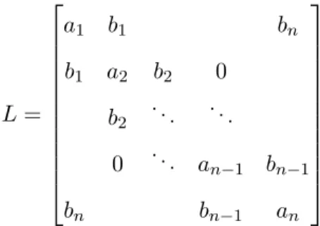
with period boundary conditions qn+1=q1. With the notationak =−12pk, bk = 12e
1
eigenvalues of the matrix
L=
a1 b1 bn
b1 a2 b2 0
b2 . .. . ..
0 . .. an−1 bn−1
bn bn−1 an
are first integrals of the system. It can be shown that the system is completely integrable. We consider the case whenn= 3 with initial conditions p1=−1.5, p2 = 1, p3= 0.5, and q1 = 1, q2 = 2, q3=−1
marching to time T = 100. We compare the explicit fourth-order Runge-Kutta method (RK4) with symplectic integrator collocation formulation with 5 Gauss nodes.
0 10 20 30 40 50 60 70 80 90 100
0 0.005 0.01 0.015
RK4 SDC(Gauss)
0 10 20 30 40 50 60 70 80 90 100
0 1 2 3 4 5 6 7 8×10
-5
RK4 SDC(Gauss)
Figure 2.1: Errors of solutions and first integrals for RK4 and Gauss collocation formulation method
From Figure 2.1, we see that the error of the solution by RK4 grows quadratically, where the error of the collocation formulation only grows linearly. For the conservation law, the error by RK4 grows linearly, whereas the error by collocation formulation doesn’t seem to grow.
2.2.2 Deferred correction
Assume we have a provisional solution ey, the error is measured by the residual function
(t) :=y0+
ˆ t
0 e
f(τ,y)e dτ−y(t).e (2.2.3)
Define the error function as
δ(t) :=y(t)−y(t).e
Restricting the error function in finite dimensional polynomial space, then we have the collocation formulation of the error equation
e
δ(t) = ˆ t
0 e
f(τ,ye+eδ)−fe(τ,y)e dτ+(t). (2.2.4)
By some algebra, locally we have
e
δ(tn+1) =eδ(tn) +
ˆ tn+1
tn
e
f(τ,ye+eδ)−fe(τ,y)e dτ+(tn+1)−(tn).
To solve the error equation efficiently, low-order methods are used for approximation. For stiff system, implicit methods, such as backward Euler’s method is used so that
e
δ(tn+1)≈δ(te n) + ∆tn[fe(tn+1,ye+eδ)−fe(tn+1,y)] +e (tn+1)−(tn). (2.2.5)
By linear implicit approximation, Eq. (2.2.5) can be solved by
e
δ(tn+1)≈δ(te n) + ∆tn
∂f(te n+1, e
y)
∂y δ(te n+1) +(tn+1)−(tn). (2.2.6)
For non-stiff system, we use explicit methods, such as forward Euler’s method,
e
δ(tn+1)≈eδ(tn) + ∆tn[fe(tn, e
y+eδ)−fe(tn, e
y)] +(tn+1)−(tn). (2.2.7)
The error is added to the provisional solution until the certain threshold is reached.
Trapezoidal’s rule, we have
e
δ(tn+1)≈δ(te n) +
∆tn
2 [(fe(tn,ey+δ)e −f(te n,y)) + (e fe(tn+1,ye+eδ)−fe(tn+1,y)] +e (tn+1)−(tn).
However, the performance of deferred correction by higher-order preconditioners is not necessarily better. We will discuss it later.
2.2.3 Perspective of linear algebra
To explore the properties of deferred correction and improve its performance, it is helpful to reformulate the problem in terms of linear algebra language. First, we give some notations, denote
Y0=
y(0) · · · y(0)
T
,
Y=
e
y(t1) · · · ey(tm) T
,
F(Y) =
e
f(t1,ey) · · · fe(tm,ey) T
.
In addition, define the normalized spectral integral matrixS such that
∆t[S]i,j =
ˆ ti
0
`j(s) ds,
where the integral can be analytically precomputed. Then we have
∆tS(i,:)·F(Y) = ˆ ti
0 e
f(τ,y)e dτ.
Euler’s method, we have
∆tSe=
∆t0 0 0 . . . 0
∆t0 ∆t1 0 . . . 0
∆t0 ∆t1 ∆t2 . . . 0
..
. ... . .. ... ... ∆t0 ∆t1 ∆t2 . . . ∆tm−1
.
Acting the integration matrix on the function gives us the right-hand rule of the Riemann sum
∆tS(i,e :)·F(Y) = i−1 X j=0
∆tjfe(tj+1,y).e
For forward Euler’s method, we have
e S=
0 0 0 . . . 0
∆t1 0 0 . . . 0
∆t1 ∆t2 0 . . . 0
..
. ... . .. . .. ... ∆t1 ∆t2 . . . ∆tm−1 0 .
Acting the integration matrix on the function gives us the left-hand rule of the Riemann sum
∆tS(i,e :)·F(Y) = i−1 X j=1
∆tjfe(tj,y).e
With the setup, the collocation formulation can be written in the matrix form
Y=Y0+ ∆tSF(Y). (2.2.8)
To solve the collocation equation is equivalent to the following root-finding problem:
Denote the provisional solution as Ye and define the error function as
δ=Y−Ye.
Substitute the relationship into the equation, we have
δ= ∆tS[F(Ye +δ)−F(Ye)] +Y0+ ∆tSF(Ye)−Ye.
Directly solving the equation is very expensive, therefore the low-order approximation is used
e
δ= ∆tS[eF(Ye +δe)−F(Ye)] +Y0+ ∆tSF(Ye)−Ye. (2.2.9)
Define the functionHe(Ye) as by solving the approximated error function with provisional solution e
Y, the deferred correction approach can be viewed as finding the roots of the nonlinear system
e
H(Ye) =0
by a fixed point iteration
Y[n+1]=Y[n]+
e
H(Y[n])
. Applying the implicit function theorem, it can be verified that the system is preconditioned
J
e
H(Ye) =−(I−∆tSeJF(Ye))−1(I−∆tSJF(Ye)).
Since the preconditionerI−∆tSeJF(Ye)has the low-triangular shape, we refer this as thetriangular
preconditioner.
in Eqs. (2.2.5) and (2.2.7). By using the forward Euler’s method, we have the linear system e
δ(t1)
e
δ(t2) e
δ(t3)
.. .
e
δ(tm) =
0 0 0 . . . 0
∆t1 0 0 . . . 0
∆t1 ∆t2 0 . . . 0
..
. ... . .. . .. ... ∆t1 ∆t2 . . . ∆tm−1 0 e
f(t1,y(te 1) +δ(te 1))−fe(t1,ey(t1)) e
f(t2,y(te 2) +δ(te 2))−fe(t2,ey(t2)) e
f(t3,y(te 3) +δ(te 3))−fe(t3,ey(t3))
.. .
e
f(tm,ey(tm) +eδ(tm))−fe(tm,y(te m)) +
(t1)
(t2)
(t3)
.. . (tm)
.
From here, we can easily recognize the error function can be solved by Eq. (2.2.7) fromt1 to tm.
Similarly, using the backward Euler’s method gives us the linear system
e
δ(t1) e
δ(t2) e
δ(t3)
.. .
e
δ(tm) =
∆t1 0 0 . . . 0
∆t1 ∆t2 0 . . . 0
∆t1 ∆t2 ∆t3 . . . 0
..
. ... . .. . .. ... ∆t1 ∆t2 . . . ∆tm−1 ∆tm
e
f(t1,y(te 1) +δ(te 1))−fe(t1,y(te 1)) e
f(t2,y(te 2) +δ(te 2))−fe(t2,y(te 2)) e
f(t3,y(te 3) +δ(te 3))−fe(t3,y(te 3))
.. .
e
f(tm,ey(tm) +eδ(tm))−fe(tm,y(te m)) +
(t1)
(t2)
(t3)
.. . (tm)
.
It is also recognized that the error equation can be solved by Eq. (2.2.5).
Remark 2.2.4. We consider a general case how Eq. (2.2.9) can be solved for PDEs. Consider the 1-dimensional parabolic PDE of the form
ut(x, t) =a(x)uxx(x, t) +b(x)ux(x, t) +c(x)u(x, t) +f(x, t)
with appropriate initial and boundary conditions. Integrate it with time, we have
u(x, t) =u0(x) +
ˆ t
0
a(x)uxx(x, s) +b(x)ux(x, s) +c(x)u(x, s) +f(x, s) ds
With approximated solution eu(x, t), we define the residual function as
(x, t) =u0(x) +
ˆ t
0
Then the error equation can be derived to satisfy
δ(x, t) = ˆ t
0
a(x)δxx(x, s) +b(x)δx(x, s) +c(x)δ(x, s) ds
with zero initial condition and also some kind of zero boundary conditions if exact boundary conditions are used. Restricting the solution in the finite-dimensional polynomial space, the collocation of error equation can be written as
e
δ(x, t) = ˆ t
0
a(x)eδxx(x, s) +b(x)δex(x, s) +c(x)eδ(x, s) ds
By backward Euler’s method, in each iteration, we have to solve
e
δ(x, tn+1) =eδ(x, tn) +a(x)eδxx(x, tn+1) +b(x)δex(x, tn+1) +c(x)eδ(x, tn+1).
A fast recursive solver can be employed with a capability of general boundary conditions to efficiently solve the equation adaptively. We leave the details of the algorithm in Chapter 3.1.
2.2.4 Krylov deferred correction
In the stiff problems, the order reduction becomes very severe, especially with increasements of the number of nodes. Motivated by the challenges caused by the stiffness, one remedy is to apply Krylov subspace methods proposed by Huang and his collaborators [43]. Instead of accepting the solution from simply fixed iteration, the optimal solutions are searched in the Krylov subspace. In detail, the Newton-Krylov method is applied to solve the nonlinear system
e
H(Ye) =0.
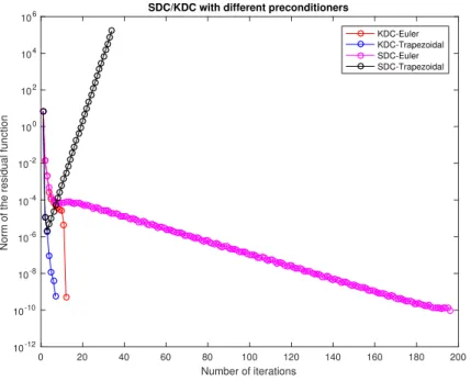
Example 2.2.2. We consider a simple problem
~y0(t) =~p0(t)−B(~y(t)−~p(t)), ~y(0) =~p(0),
where ~y(t) and ~p(t) are vectors of dimension N. The exact solution is given by~y(t) =~p(t). The matrix B is constructed by
B =UTΛU
where U is a randomly generated orthogonal matrix, and Λis a diagonal matrix whose diagonal entries{λi}Ni=1 are all positive. Forp(t), we choose the~ ith component ascos(t+αi) with phase
parameter αi = 2Nπ. We set the dimension of the system to 10, and use 10 Lobatto nodes in the
simulation. We use ∆t= 0.1and study one time step. We setλ1 =O(107)and the rest to the order
of O(10−1). The result is plotted in Figure 2.2.
0 20 40 60 80 100 120 140 160 180 200
Number of iterations 10-12
10-10 10-8 10-6 10-4 10-2 100 102 104 106
Norm of the residual function
SDC/KDC with different preconditioners
KDC-Euler KDC-Trapezoidal SDC-Euler SDC-Trapezoidal
Figure 2.2: Deferred correction for the linear multimode problem
subspace, it takes 12 iterations to converge for Euler’s preconditioning and 7 iterations for Trape-zoidal’s preconditioning. We can see that the convergence is significantly accelerated in this problem. In addition, although the Trapezoidal’s rule is not stable for SDC, it converges efficiently for KDC. 2.3 Convergence analysis
In this section, we analyze the convergence of deferred correction for ODEs. The emphasize is on the stiff systems, in which order reduction is observed.
The standard reduction is used [91]. Start from the original problem y0(t) = f(t, y) and let
y0(t) denote a particular solution of the ODE we are interested in. If we make the substitution
y(t) =y0(t) +u(t), then by linearization, we consider the problemu0(t) =A(t)u(t). We then freeze
the coefficient by setting A=A(t0) for somet0 of interest. The idea here is that instability and
stiffness are fundamentally transient phenomena, which may appear near some time t0 and not
others. The result is the constant coefficient linear problem. By diagonaliazation, we focus on the scalar problemu0(t) =λu(t).
Remark 2.3.1. This argument is not always true, Trefethen [91] discuss the potential failures of the approach. Nevertheless, it has achieved lots of success in applications.
In the scalar constant coefficient problem, we have the collocation formulation
Y =Y0+ ∆tλSY.
By Picard’s iteration, the solution is updated by Neumann series
Y[n+1] =CY[n]+b,
where
Cpic= ∆tλS,
bpic=Y0.
methods for the problem is also equivalent to apply the Neumann series, but with preconditioning technique so that
Cdc =I−(I−∆tλS)e −1(I−∆tλS),
bdc = (I−∆tλS)e −1Y0.
Then it is sufficient to analyze the eigenstructure of the convergence matrix C if it is diagonalizable.
Theorem 2.3.1. For linear ODE IVPs, the deferred correction iterations are convergent if and only if the spectral radius ρ(C) (the supremum among the absolute values of all the eigenvalues) of the correction matrixC is less than 1.
Motivated by the theorem, we define the “convergence region" to measure when the deferred correction methods are convergent for linear problems:
Definition 2.3.1. For linear ODE IVPs, we define the “convergence region" Ω of a deferred correction method as Ω ={λ∆t: ρ(C(λ∆t)) <1, λ∈ C}. The method is called “A-convergent"
if Ω contains the left half complex plane. It is called “L-convergent" if it is “A-convergent" and lim|λ∆t|→∞ρ(C(λ∆t))→0for λ∆t on the left half complex plane.
We find it very challenging to analyze in general scenario. To reduce the burden, we begin by considering asymptotic cases, then we numerically compute the contour lines of ρ(C) to give an intuitive explanation.
2.3.1 Non-stiff systems For the case λis small, recall
Cdc = (I−∆tλS)e −1∆tλ(Se−S).
We also obtain a factor of ∆tλ in each iteration. Furthermore, we expect the low frequencies errors are reduced better than Picard’s iteration due to the term Se−S. The argument is verified in the
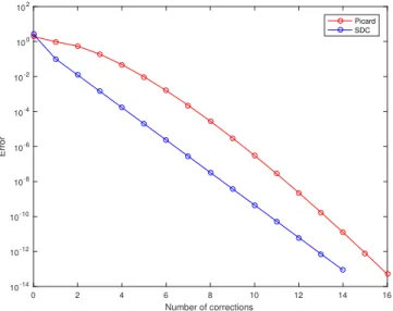
Example 2.3.1. Consider the ODE
(y(t)−cos(t))0 =λ(y(t)−cos(t)), y0 = 1.
Apparently the analytical solution is y(t) = cos(t). This toy example can be used to understand the stiffness of the system and we will use it over and over again in the rest of the thesis. For non-stiff system, we set T = 1, λ= 1 with 10 Lobatto nodes. The final error is1.08×10−11. From
the Figure 2.3, we can see that the SDC converges slightly faster than Picard’s iteration, but their convergence rate is about the same.
0 2 4 6 8 10 12 14 16
Number of corrections 10-14
10-12 10-10 10-8 10-6 10-4 10-2 100 102
Error
Picard SDC
Figure 2.3: Comparison of deferred correction and Picard iteration
Remark 2.3.2. It is natural to wonder if the convergence can be accelerated by higher order preconditioners. It is shown in [40] if the nodes are chosen to be uniform, then in non-stiff system, the higher-order convergence is obtained by Runge-Kutta methods. We also obtain the similar results for the Trapezoidal’s rule preconditioner.
2.3.2 Stiff systems
the backward Euler’s method with Gauss nodes, in the strong stiff case such thatRe(λ)→ −∞, we want to understand the eigenstructure of the matrix
Cdc∼I−Se−1S.
With first glance, we notice that λ and∆t are canceled out, which explains the reduction of the order. The eigenvalues of the matrix are numerically solved to have a deeper insight. The result is summarized in Table 2.1.
n 2 3 4 5 6 7 8
0.3170 0.4210 0.5610 0.6653 0.7420 0.7998 0.8448
n 9 10 11 12 13 14 15
0.8805 0.9096 0.9337 0.9540 0.9713 0.9861 0.9991
n 16 17 18 19 20 25 50
1.0105 1.0205 1.0295 1.0375 1.0448 1.0724 1.1280
Table 2.1: ρ(I−Se−1S) for different numbers of Gauss nodes, stiff case,SDC.
With increasements of the number of nodes, we find out the order reduction becomes more severe. In particular, in the strong stiff system, the SDC with more than 15 points will diverge. We have seen advantages in convergence by using higher-order preconditioners in the non-stiff cases, however, such successes are usually not observed in the stiff system. We analyze it in the same way and numerically calculate eigenvalues of the convergence matrix and show the results in the Table 2.2.
n 3 4 5 6 7 8 9
|λ|max 0.3333 0.6180 0.8934 1.1658 1.4370 1.7076 1.9780
n 10 11 12 13 14 15 16
|λ|max 2.2482 2.5183 2.7884 3.0585 3.3285 3.5986 3.8687
n 17 18 19 20 21 25 50
|λ|max 4.1388 4.4089 4.6789 4.9490 5.2191 6.2995 13.0530
Table 2.2: ρ(C) of SDC-Lobatto-T, strongly stiff limit case.
We observe that |λ|max soon grows bigger than 1, with even 6 nodes, which explains the failure
of the Trapezoidal’s rule in the stiff case.
theorem.
Theorem 2.3.2. For the yp-formulation with uniform nodes, when |λ∆t| → ∞, the correction matrix Se−1S−I has eigenvalues equal to zero; and its Jordan canonical form consists of one Jordan
block.
Remark 2.3.3. The uniform nodes discretization seem to have better convergence. However, it should be avoided with a large number of nodes due to the well-known Runge phenomenon.
Finally, if the left endpoint is included, then the simple asymptotic relation Cdc ∼ I−Se−1S
cannot be hold since the first row of Se and S are zeros. In case, we re-write the matrix in the
following form:
S=
01×1 01×(m−1)
S21 S22
whereS21∈R(m−1)×1 and S22∈R(m−1)×(m−1). Similarly, denote
e
S=
01×1 01×(m−1)
e
S21 Se22 .
Apply Woodbury matrix identity, we duduce that
C=
0 0
(I−∆tλSe22−1∆tλ(S21−Se21) I−(I−∆tλSe22)−1(I−∆tλS22) .
Hence it is sufficiently to analyze the submatrixI−(I−∆tλSe22)−1(I−∆tλS22).
2.3.3 General cases
In general cases, we numerically compute the contour lines of the convergence of correction matrix in terms of different values of∆tλ. We focus on the Euler’s method since the Trapezoidal’s rule seem to be unstable in a stiff system.
when we calculate the dynamics of Schrödinger type equations. Similar results can be shown for different type quadratures. One interesting observation is that the yp-formulation with less than 5 uniform nodes is L-convergent [84].
0.3 0.4 0.5 0.5 0.6 0.6 0.6 0.6 0.7 0.7 0.7 0.7 0.8 0.8 0.8 0.8 0.8 0.8 0.9 0.9 0.9 0.9 1 1 1 1.1 1.1 1.1
-40 -30 -20 -10 0 10 20 30 40
x -40 -30 -20 -10 0 10 20 30 40 y 0.30.4 0.5 0.6 0.7 0.7 0.8 0.8 0.8 0.8 0.9 0.9 0.9 1 1 1 1.1 1.1 1.1 1.1 1.1 1.2 1.2 1.2 1.2
-100 -80 -60 -40 -20 0 20 40 60 80 100
x -100 -80 -60 -40 -20 0 20 40 60 80 100 y
Figure 2.4: Contour lines ofρ(C(λ∆t))for m= 5 and m= 10for SDC,λ=x+iy
2.4 Diagonal preconditioners
In this section, we introduce a new class of diagonal preconditioners. The new preconditioner is very stable and easy to parallelize.
In order to achieve the local parallelization, we need to decouple the dependencies between the current node and the previous nodes. Hence, we update the error directly from the initial node. For stiff systems, with backward Euler’s method, we have
e
δ(tn+1)≈tn+1[f(te n+1,ye+δ)e −f(te n+1,ey)] +(tn+1).
For non-stiff systems, with forward Euler’s method, we have
e
δ(tn+1)≈tn+1[fe(t0,ye+δ)e −f(te 0,y)] +e (tn+1).
form, the backward Euler’s integration matrix now becomes diagonal
e
S =
∆t0 0 0 . . . 0
0 ∆t1 0 . . . 0
0 0 ∆t2 . . . 0
..
. ... . .. ... ... 0 0 0 . . . ∆tm−1
.
Correspondingly, the preconditioner I −∆tSeJF(Ye) also becomes diagonal. For this reason, we
refer this as the diagonal preconditioner. It is straightforward to generalize it to higher-order preconditioning techniques. For example, with Trapezoidal’s rule, we have
e
δ(tn+1)≈
tn+1
2 [(fe(t0,ye+δ)e −fe(t0,ey)) + (fe(tn+1,ye+eδ)−fe(tn+1,y)] +e (tn+1).
To accelerate the convergence, one could also adopt the KDC framework with diagonal preconditioners. To understand the behavior of this new class of preconditioners, we apply the similar analysis as in the last section. For non-stiff systems, the results are pretty similar. We focus on the stiff systems. For this particular type of preconditioners, in the strong stiff case, we are able to provide some analytical results. Assuming∆t= 1 andλ= 1
, where→0 and we want to calculate the
eigenvalues of the preconditioned system
A=
I+1 Se
−1
I+1 S
= (I+S)e −1(I+S).
Assume µis the eigenvalue of A, we deduce that
AF=µF
We take the asymptotic expansion with first two terms, assume that
F∼F0+F1,
µ∼µ0+µ1.
Substitute those into the equation,
(I+S)(F0+F1) = (µ0+µ1)(I+S)(e F0+F1). (2.4.1)
By matching the O(1)terms,
SF0 =µ0SeF0.
Matching theO() yields
F0+SF1 =µ0SeF1+µ0F0+µ1SeF0.
We are able to provide following theorems regarding the backward Euler’s method and Trape-zoidal’s rule.
Theorem 2.4.1. If Se is discretized by backward Euler’s method, then
[µ0]n= n1
[F0]n= [tn−1 1, . . . , tn−m 1]T.
If endpoints are not included, then
[µ1]n= 0,
[F1]n=−(n−1)2[tn−1 2, . . . , tn−m 2]T.