Shortest Alternate Path Discovery through Recursive Bounding Box Pruning

http://www.scirp.org/journal/jtts ISSN Online: 2160-0481

ISSN Print: 2160-0473

Shortest Alternate Path

Discovery through Recursive Bounding Box

Pruning

Rajendra S. Parmar

, Bhushan H. Trivedi

1_{Gujarat Technology University (GTU), Ahmedabad, India}

2_{Gujarat Law Society Institute of Computer Technology, Ahmedabad, India}

Abstract

Congestion is a dynamic phenomenon and hence efficiently computing alter-nate shortest route can only help expedite decongestion. This research is aimed to efficiently compute shortest path for road traffic network so that congestion can be eased resulting in reduced CO2 emission and improved economy. Congestion detection is achieved after evaluating road capacity and road occupancy. Congestion index, a ratio of road occupancy to road capacity is computed, congestion index higher than 0.6 necessitates computation of al-ternate shortest route. Various algorithms offer shortest alal-ternate route. The paper discusses minimization of graph based by removing redundant nodes which don’t play a role in computation of shortest path. The proposal is based on continuous definition of a bounding box every time a next neighboring node is considered. This reduces maximum number of contentious nodes re-peatedly and optimizes the network. The algorithm is deployed from both the ends sequentially to ensure zero error and validate the shortest path discovery. While discovering shortest path, the algorithm also offers an array of shortest path in ascending order of the path length. However, vehicular traffic exhibits network duality viz. static and dynamic network graphs. Shortest route for static distance graph is pre-computed and stored for look-up, alternate short-est path based on assignment of congshort-estion levels to edge weights is triggered by congestion index. The research also supports directed graphs to address traffic rules for lanes having unidirectional and bidirectional traffic.

Keywords

Bounding Box Pruning, Geometric Containers, Shortest Alternate Path, Shortest Path, Vehicular Traffic, Vehicular Congestion, Detection System, Vehicular Congestion Detection System

How to cite this paper: Parmar, R.S. and Trivedi, B.H. (2017) Shortest Alternate Path Discovery through Recursive Bounding Box Pruning. Journal of Transportation Tech-nologies, 7, 167-180.

https://doi.org/10.4236/jtts.2017.72012

Received: February 22, 2017 Accepted: April 15, 2017 Published: April 18, 2017

Copyright © 2017 by authors and Scientific Research Publishing Inc. This work is licensed under the Creative Commons Attribution International License (CC BY 4.0).

http://creativecommons.org/licenses/by/4.0/

1. Introduction

The paper proposes network optimization or graph optimization technique th- rough pruning by bounding box. This is a recursive methodology which conti-nuously reduces redundant nodes and edges of a given network which are not contentious in computation. Section II, discusses related work where shortest path algorithms are discussed. This section also discusses various network mi-nimization techniques. Section III introduces Definition & Terminology. Here road capacity, road occupancy, congestion index are discussed to build the frame work of the solution. Section IV is the proposition and methodology to minim-ize the network scope. This section defines network representation and follows it with algorithm explaining the importance of evaluation from both the nodes (start node and end node) under consideration. Section V is Results and Com-parison clearly validating the results achieved while addressing the network from start or end node. The section also discusses the maximum computing cost with this approach. Section VI is Future work, when angled bounding box approach can further improve the results.

It is important to understand vehicular network duality. Present network al-gorithms and strategies consider network with edges representing weights and nodes as identity entity with nil weight. The data networks are treated as scalar network whereas spatial road networks are vector networks. Vehicular network exhibits duality. There are two vehicular networks: 1) Static distance network; 2) Dynamically changing traffic network which changes with congestion. A graph with distances is created and shortest path is evaluated from every node to the remaining nodes. The pre-computed shortest path is available in the infrastruc-ture database. However, during congestion, the travel time of road segment in-creases. A road segment with shorter distance may take longer to travel than the longer road segment. The dynamic graph edge weight is dynamically updated, and continuously computed. Secondly, data travels at speed of light and hence during congestion, choosing alternate paths does not add appreciable delay. Also data networks are huge, offering multiple alternate routes without appreciable degradation in response time. Whereas vehicular speeds are infinitesimally less compared to speed of light and hence shortest alternate route selection requires judicious decision since it is more challenging.

2. Related Work

[1] Premier contribution in path finding algorithm is done by A*, BFS, Dijkstra’s algorithm, HPA* and LPA* which are discussed below:

2.1. Algorithms

2) BFS

[2] BFS does not take advantage of knowledge or heuristics. For a graph G = (V, E), BFS travels edges from start to end node ensuring minimum number of edges to reach the goal. Algorithm complexity varies between O (V ) and O

( 2

V ).

3) Dijkstra’s algorithm

[2] The algorithm iteratively selects nodes u ε V-S, is “greedy” algorithm. Maximum computation cost is O ( E +V Log V ). Dijkstra’s algorithm

discov-ers shortest paths from one node to all the other nodes, however, when one needs to discover shortest path between two given nodes, there are other fitting solutions.

4) Hierarchical path-finding A*

[2] HPA* A low resolution 2D grid is placed on graph. Every node in the new grid is a cluster. The algorithm simplifies the graph to make efficient computa-tions.

5) Lifelong Planning A* (LPA*)

[2] LPA best used where the graph changes dynamically. S represents vertices. The programming functions used are a) succ(s) of vertex s of S; b) pred(s) pre-decessors of vertex s of S; c) 3. 0 < c (s, s’) ≤ α cost of moving from vertex s to vertex s’.

( )

( )

(

( ) (

)

)

0

min , otherwise

start

s pred s

if s s

g s

g s c s s

′∈ =  ∗ _{=  ′ ′} ∗ + 

2.2. Pruning Techniques

1) [3] Deals with dynamically changing edge weights. A graph is broken into containers and the size of the containers keep on changing. If the container is large it losses the advantage and if too small, it may not offer best results. Opti-mizing size of the container is achieved in this paper.

2) [4] Proposed combination of two techniques: Jump Point Search (JPS) and geometric containers. On uniform grid, JPS defines a canonical ordering to mi-nimize search. The search begins at the central node of the graph and proceeds in the directions of the arrows. To begin with it takes the only the diagonal route and then only cardinal moves. Instead of evaluating every node on its way to shortest path discovery, it jumps along straight lines towards the goal thus sav-ing computation cost of addsav-ing and removsav-ing a node.

3) [5] Geometric Containers is a class of approach mapped to metric spaces. The edges reachable to the goal are placed in a container. Then only those edges are evaluated which are inside the container rest are pruned.

4) [6] A swamp is a group of nodes which are not evaluated while exploring shortest path. Ignoring swamps, does not affect the accuracy of the shortest path search. Swamps are a geometric container yielding no results, thus ignored to improve computational efficiencies.

node evaluation. However, the method through extensive experiments discovers optimal number of nodes empirically by clipping containers.

6) [8] A reach value is associated with every node. If the reach value of the node is not in the vicinity of the start or end node, it is ignored.

7) [9] A bounding box is defined for each edge. Every node is then queried to check if it is contained in the bounding box or not. This is done by evaluating if there is a valid path to the end node. There is forward and backward pre-com- putation in this approach.

8) [10] Proposed several concepts to create minimally pruned graph. Disk Centered Tail-DCT takes an edge end as the entre and a minimum radius circle is drawn encompassing all the nodes connected to this node. The concept is known as disk centered tail. Ellipse is an extension of DCT where the ellipse has foci of u and v. Angular Sectors-AS is selected by choosing a node on the left and right of the edge node u. The AS is formed by left node, edge node and right node. AS have no bounds which does not achieve effective pruning. So AS is bounded by DCT and generates CT-circular sectors. Smallest enclosing disk- SED is unique disk which has smallest area that includes all the points. Smallest Enclosing Ellipse-SEE is generated from SED the way Ellipse is generated from DCT. Bounding Box-BB (Axes Parallel Rectangle) encloses area bounded by four coordinates of two points. Edge Parallel Rectangle-EPR is a situation where the rectangle is parallel to the edge and not the axes. Intersection of Rectangle-IR offers even smaller container. Here the axes parallel and edge parallel rectangles are intersected.

3. Definitions/Terminology

This section discusses algorithms to discover shortest alternative route with minimum computing cost. The computing cost is evaluated based on travel dis-tance and time to travel. The alternate route is sought as follows:

1) Compute road capacity from infrastructure database-RC. 2) Compute road occupancy-RO.

3) Compute congestion index (RO/RC).

4) If congestion index is high, (>0.6), evaluate alternate shortest route.

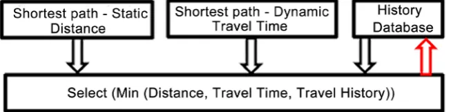
Alternate routes are selected from amongst distance route, alternate shortest route based on congestion and knowledge or history database. Figure 1 depicts the logical flow. The selected alternate route is then logged into the history da-tabase for future reference.

3.1. Road Capacity (Infrastructure Database-Big Data)

[11] A test vehicle equipped with GPS capable application software. The vehicle traverses through the city capturing infrastructure parameters. Latitude, Longi-tudes are captured automatically by GPS, average achievable speed on road seg-ment is a secondary parameter derived from time stamped latitude and longi-tude whereas road name, number of lanes, presence of traffic signals and con-verging road segments are manually input to the application. This information provides road capacity and time to travel on the road segment.

*

RC=L N (1)

L = Length of road segment; N = Number of lanes

Normal travel time of the road segment is computed from the time stamped distance coordinates.

3.2. Road Occupancy

A GPS capable device with application software is attached with each vehicle, which transmits vehicle location. The vehicle ID and GPS device are paired to create a unique identification providing manufacturer, model, fuel type and eco- nomy, area, length and breadth. The location coordinate data is time stamped. Consecutive time stamped location coordinates provides speed and mean veloc-ity. Data acquired from different vehicles are mapped to road segments with ve-hicle area to provide RO (road occupancy).

( )

RO=

∑

3.3. Congestion Index

Congestion index-CI is a parameter of significance to trigger computation of al-ternate routes. CI defines degree of congestion, is a ratio of road occupancy to road capacity. Road capacity is extracted from the infrastructure database, whe- reas road occupancy is computed from vehicle detection.

4. Shortest Alternate Route

The steps are:

1) Creation of network graph of a city with nodes (Latitude/Longitude) and edge weights as distance.

2) Represent the data graphically.

3) Describe the graph through a tabular matrix. Create a table of nodes, coor-dinates, distance to origin, distance to destination, total distance.

4) Bounding Box, the network optimization schema.

4.1. Representation—Tabular & Graphical

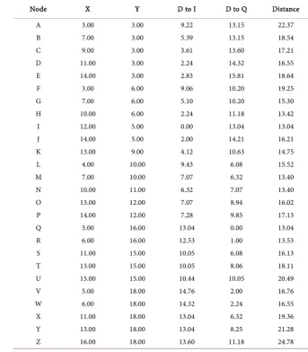
Coordinates of nodes (traffic junctions), each nodes distance from the two nodes in consideration (starting and end node) and the total distance of the node from the two nodes is listed in Table 1:

marked as edge weights.

4.2. Bounding Box—Concept

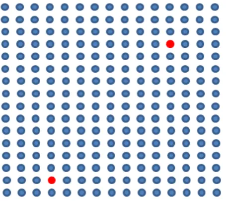
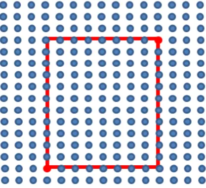
Consider a network with 225 nodes as shown in Figure 3. Figure 4 shows a bounding box rectangle is created between start node and end node. The nodes embedded in the rectangle are considered and all the other nodes are ignored thus reducing redundant computation. Defining a bounding box considerably reduces the network to 108 nodes there by reducing the scope of the network and reducing the computation cost & time.

4.3. Heuristics/Hypothesis

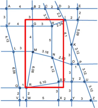
The two dimensional location coordinates in road transport network help in understanding if the approaching node is converging to the end node or not. A start node and end node is defined. A bounding box is created between start node and end node. From start node, all connected edges are tested to get a list of connected nodes. For every connected node the distance d is:

Table 1. Tabular representation.

Node X Y D to I D to Q Distance

A 3.00 3.00 9.22 13.15 22.37

B 7.00 3.00 5.39 13.15 18.54

C 9.00 3.00 3.61 13.60 17.21

D 11.00 3.00 2.24 14.32 16.55

E 14.00 3.00 2.83 15.81 18.64

F 3.00 6.00 9.06 10.20 19.25

G 7.00 6.00 5.10 10.20 15.30

H 10.00 6.00 2.24 11.18 13.42

I 12.00 5.00 0.00 13.04 13.04

J 14.00 5.00 2.00 14.21 16.21

K 13.00 9.00 4.12 10.63 14.75

L 4.00 10.00 9.43 6.08 15.52

M 7.00 10.00 7.07 6.32 13.40

N 10.00 11.00 6.32 7.07 13.40

O 13.00 12.00 7.07 8.94 16.02

P 14.00 12.00 7.28 9.85 17.13

Q 5.00 16.00 13.04 0.00 13.04

R 6.00 16.00 12.53 1.00 13.53

S 11.00 15.00 10.05 6.08 16.13

T 13.00 15.00 10.05 8.06 18.11

U 15.00 15.00 10.44 10.05 20.49

V 5.00 18.00 14.76 2.00 16.76

W 6.00 18.00 14.32 2.24 16.55

X 11.00 18.00 13.04 6.32 19.36

Y 13.00 18.00 13.04 8.25 21.28

Figure 2. Graphical representation.

Figure 3. Consider 15 × 15 = 225 nods.

(

)

d= Edge weight Cartesian distance to end node+ (3)

From amongst the node, final selected distance d is selected based on:

(

)

{

}

d= Min Edge weight+Cartesian distance to end node (4)

Figure 4. Bounding box reduces 108 nodes.

is sorted in ascending order based on distance or cost of travel. This provides al-ternate shortest route as well as next best routes. The same process is followed by swapping start and end node and shortest route array is obtained. The two ar-rays are merged to get best results. In case the algorithm fails to discover shortest route, the bounding box is extended to expand the scope of the search.

4.4. Algorithm

Bounding box (Start Node, End Node) Find connected nodes to start node

Compute Distance for all nodes = (Edge weight + Cartesian distance to end node)

Next Node = Min (Compute Distance)

Store other nodes in pending list (Travelled nodes, Distance travelled) Start node = Next node

IF (Start node ≠ End node) Go to step 1

Store result (Traveled nodes, Travelled Distance) If Pending list = Null) Step 2

Pick up from Pending list Start node = Selected node Go to step 1

Step 2

If (Switch done = True) Step 3 Switch done = True

Swap (Start node, End node) Go to Step 1

Step 3

If (Result ≠ Null) Go to Step 4

Switch = False Go to Step 1 Step 4

Evaluate Min (Result) End

Moving from Start Node Q to End Node I Bounding box (Q, I)Figure 5

Within a bounding box (Q, I), Q is only connected to R Bounding box (R, I)Figure 6

R is connected to M & S

Figure 5. Moving Q to I; bounding box (Q, I).

R → M → I 13.15 R → S → I 15.12

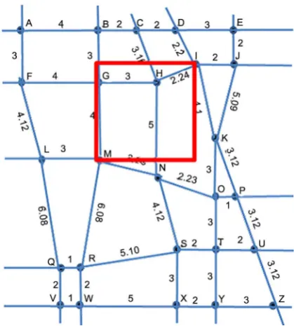
For now M is considered; S is stored for subsequent consideration Bounding box (M, I)Figure 7

M connects to G

Bounding box (G, I)Figure 8 G connects to H

Bounding box (H, I)Figure 8

Figure 7. Moving Q to I; bounding box (M, I), S

subse-quent consideration.

H connects to I Route QRMGHI 16.32 Open S

Bounding box (S, I)Figure 9 S is isolated, disconnected

Bounding box is increased Figure 10 S connects to N

Bounding box (N, I)Figure 11 N connects to H

Figure 9. Moving Q to I; bounding box (S, I).

Figure 11. Moving Q to I; bounding box (N, I).

Figure 13. Bounding box consideration of approx 89 nods.

Figure 14. Bounding box consideration of approx 64.

Bounding box (H, I)Figure 11 H connects to I

Route QRSNHI 17.46

5. Results

Starting from Q to I the shortest routes are QRMGHI 16.32 units and QRSNHI 17.46 units. Starting from I the shortest routes are IHGMRQ 16.32 units, IHNSRQ 17.46 units and IHNMRQ 17.48 units.

Summing up we get three routesQRMGHI16.32 units, QRSNHI17.46 units and QRMNHI17.48 units.

plotted in Figure 12. The maximum computing cost is:

Maximum computing cost=7 * 2N (5)

Further reduction is possible when angled bounding box is employed. Instead of the bounding box aligned to the axes, it is proposed to tilt it at an angle such that one pair of parallel sides of bounding box is parallel to the axes connecting start and end nodes. For best results, the width of the rectangle (perpendicular to the axes of start and end node) is kept minimum. If there are no neighboring nodes OR the algorithm fails to find the shortest path, then the rectangle is wi-dened till the algorithm finds neighboring node OR shortest path. This is dem-onstrated in Figure 13 and Figure 14.

References

[1] Parmar, R.S. and Trivedi, B. (2016) Shortest Route—Domain Dependent, Vectored Approach to Create Highly Optimized Network for Road Traffic. International Journal of Traffic and Transportation Engineering, 5, 1-9.

[2] Zarembo, I. and Kodors, S. (2013) Path Finding Algorithm Efficiency Analysis in 2D Grid. Proceedings of the 9th International Scientific and Practical Conference, Volume 1,20-22 June 2013.

[3] Wagnera, D., Willhalma, T. and Zaroliagis, C. (2004) Dynamic Shortest Paths con-tainers. Electronic Notes in Theoretical Computer Science, 92, 65-85.

www.elsevier.com/locate/entcs

[4] Harabor, D.D. and Grastien, A. (2011) Online Graph Pruning for Path Finding on Grid Maps. AAAI Conference on Artificial Intelligence, San Francisco, 7-11 August 2011.

[5] Wagner, D., Willhalm, T. and Zaroliagis, C.D. (2005) Geometric Containers for Ef-ficient Shortest-Path Computation. Journal of Experimental Algorithmics, 10, Ar-ticle No. 1.3.

[6] Pochter, N., Zohar, A., Rosenschein, J.S. and Felner, A. (2010) Search Space Reduc-tion Using Swamp Hierarchies. AAAI Conference on Artificial Intelligence, Atlanta, 11-15 July 2010.

[7] Park, J., Moon, D. and Hwang, E. (2010) A Border Line-Based Pruning Scheme for Shortest Path Computations. KSII Transactions on Internet and Information Sys-tems, 4, 939-955.

[8] Kaplan, G.H. and Werneck, R.F. (2006) Reach for A: Efficient Point-to-Point Shortest Path Algorithms. SIAM Workshop on Algorithms Engineering and Expe-rimentation, Miami, January 2006, 41. https://doi.org/10.1137/1.9781611972863.13

[9] Rabin, S. and Sturtevant, N.R. (2016) Combining Bounding Boxes and JPS to Prune Grid Path Finding. Association for the Advancement of Artificial, Intelligence.

www.aaai.org

[10] Wagner, D. and Willhalm, T. (2003) Geometric Speed-Up Techniques for Finding Shortest Paths in Large Sparse Graphs. Universit at Karlsruhe, Institut fur Logik, Komplexit at und Deduktionssysteme, D-76128, Karlsruhe, Springer, Berlin Hei-delberg.

Submit or recommend next manuscript to SCIRP and we will provide best service for you:

Accepting pre-submission inquiries through Email, Facebook, LinkedIn, Twitter, etc. A wide selection of journals (inclusive of 9 subjects, more than 200 journals)

Providing 24-hour high-quality service User-friendly online submission system Fair and swift peer-review system

Efficient typesetting and proofreading procedure

Display of the result of downloads and visits, as well as the number of cited articles Maximum dissemination of your research work

Submit your manuscript at: http://papersubmission.scirp.org/