Analysis and Comparison of Time Replica and Time Linear Interpolation for Pilot Aided Channel Estimation in OFDM Systems

(1)

Analysis and Comparison of Time Replica and Time

Linear Interpolation for Pilot Aided Channel

Estimation in OFDM Systems

Donglin Wang

Department of Electrical and Computer Engineering, University of Calgary, Calgary, Canada Email: [email protected]

Received March 10, 2010; revised April 11, 2010; accepted May 12, 2010

Abstract

This paper analyzes and compares two time interpolators, i.e., time replica and time linear interpolator, for pilot aided channel estimation in orthogonal frequency division multiplexing (OFDM) systems. The mean square error (MSE) of two interpolators is theoretically derived for the general case. The equally spaced pilot arrangement is proposed as a special platform for these two time interpolators. Based on this proposed plat-form, the MSE of two time interpolators at the virtual pilot tones is derived analytically; moreover, the MSE of per channel estimator at the entire OFDM symbol based on per time interpolator is also derived. The ef-fectiveness of the theoretical analysis is demonstrated by numerical simulation in both the time-invariant frequency-selective channel and the time varying frequency-selective channel.

Keywords:

OFDM, Channel Estimation, Time Replica, Time Linear Interpolation, Virtual Pilots

1. Introduction

Orthogonal frequency division multiplexing (OFDM) [1-3] has been widely used in high-speed wireless com-munication systems, such as broadband wireless local area networks (WLANs) [4], wireless metropolitan area networks (WMANs) [5] and worldwide interoperability for microwave access (WIMAX) [6], due to its advan-tages of transforming frequency-selective fading chan-nels into a set of parallel flat fading sub-chanchan-nels and eliminating inter-symbol interference [7].

Channel estimation is one of the most essential tasks in compensating distortion from channels and perform-ing coherent detection in OFDM systems. Estimation is usually performed by using pilot tones [8, 9] and is based on inserting known pilot tones in each OFDM symbol, where interpolation in time-frequency grid [10] plays an important role in the estimation process. The usage of virtual pilot tones [11-13] and time interpolation can reduce the redundancy and guarantee a higher transmis-sion bit rate. Among time interpolation methods, time replica [14, 15] is widely used in time-invariant or slow time-varying channel, which is simple to implement and also efficient for subcarrier usage; time linear interpola-tion [16-18] is widely used in slow or fast time-varying channel, because it is simple to realize and usually can

give a satisfactory performance. However, some inter-esting questions are raised as follows: 1) what kind of time-varying channel is slow enough to utilize time rep-lica? 2) Conversely, what kind of time-varying channel is so fast that we have to employ time linear interpolation instead of time replica? And 3) how much does time lin-ear interpolation perform better than time replica by for a time-invariant channel?

(2)

tones is finally obtained by frequency linear interpolation [20].

This paper is organized as follows. In Section 2, the MSEs of two interpolators, i.e., time replica and time linear interpolation, are theoretically derived for the gen-eral case. In Section 3, the equally spaced pilot arrange-ment is proposed as a special platform for analyzing these two time interpolators. In Section 4, based on the proposed platform, the MSE of two time interpolators at the virtual pilot tones is derived analytically; moreover, the MSE of channel estimators at the entire OFDM symbol based on these two time interpolators is also de-rived, respectively. Numerical results are reports in Sec-tion 5, followed by conclusion in SecSec-tion 6.

Notation: g2 denotes the modulus. g2 is the 2-norm operation. Ek

{ }

g is the expectation operation

on k. Ek l,

{ }

g means the expectation on both k and l.

{ }

k

Var g means the variance on k. δm i m−, +j( )k denotes

the variation of the CSI of the kth tone from the

(

m i−

)

th OFDM symbol to the

(

m+ j

)

th OFDM symbol. δm( )k denotes the variation of the CSI of the

th

k tone from the mth OFDM symbol to the

(

m+1 th

)

OFDM symbol. emR

( )

k and

( )

L m

e k are the channel estimation errors of the mth OFDM symbol at the thk tone where time replica or time linear interpo-lation are employed for CSI estimation at the virtual pilot tones, respectively.

2. MSE of Two Time Interpolators

Assume that each OFDM symbol has N subcarriers where pilots occupy P subcarriers. Denote the set of pilot tones by I_P. By LS estimation, the CSI at pilot tones in the th

m OFDM symbol can be obtained as ( )

ˆ _{( )}

( )

m m

m

Y k H k

X k

= (1)

where X_m( )k and Y k_m( ) are the transmitted and re-ceived pilots of the mth OFDM symbol, respectively. Assuming the pilot tones X_m( )k =1 for convenience of analysis, we have

ˆ _{( )} _{( )} _{( )}

m m m

H k =H k +W k (2) where Hm( )k represents the true value and W km( ) is

a complex-valued sample of additive white Gaussian noise (AWGN) process at the mth OFDM symbol,

( )

2

( ) ~ 0,

m

W k CN σ .

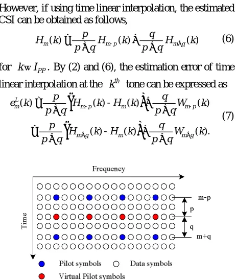
Assuming that along the time axis in Figure 1, the da-ta tones in the mth OFDM symbol correspond to the pilot tones in both the

(

m−p

)

th and the

(

m q+

)

th OFDM symbol, the CSI at the data tones in the mth OFDM symbol can be obtained by time interpolation by using the estimated CSI at the pilot tones of both the

(

m−p

)

thand the

(

m q+

)

th OFDM symbol, which is thus called the virtual pilot tones. Denote the set of vir-tual tones by IPP. In this section, we will analyze and

compare the MSE performance of two time interpolators: time replica and time linear interpolator.

2.1. Time Replica

Time replica at the virtual pilot tones in the mth sym-bol is to replicate the CSI at the pilot tones in the

(

m−p

)

th symbol,

ˆ _{( )} ˆ _{( ),}

m m p PP

H k =H ₋ k k∈I . (3) By (2) and (3), the estimation error of time replica at the thk tone can be expressed as

--

-ˆ

( ) ( ) - ( )

( ) - ( ) ( ).

R

m m p m

m p m m p

e k H k H k

H k H k W k =

= + (4) The MSE using time replica can thus be obtained as

{

}

{

}

{

}

2 2 ₂

-2 ₂

,

( ) ( ) - ( )

( ) .

R

R k m k m p m

k m p m

E e k E H k H k

E ₋ k

= = +

= +

ξ σ

δ σ

(5)

2.2. Time Linear Interpolation

However, if using time linear interpolation, the estimated CSI can be obtained as follows,

-ˆ _{( )} ˆ _{( )} ˆ _{( )}

m m p m q

p q

H k H k H k

p q p q +

= +

+ + (6)

for k∈I_PP. By (2) and (6), the estimation error of time linear interpolation at the kth tone can be expressed as

(

)

(

)

-

-( ) ( ) - ( ) ( )

( ) - ( ) ( ).

L

m m p m m p

m q m m q

p q

e k H k H k W k

p q p q

p q

H k H k W k

p q + p q +

= +

+ +

= +

+ +

(7)

[image:2.595.310.541.401.675.2]

(3)

Based on (7), the MSE of time linear interpolation can thus be obtained as

{

}

(

)

2

2 2

, , 2

2

( )

( ) ( )

.

L

L k m

m p m m m q

k

E e k

p k q k p q

E

p q p q p q

− +

=

  ₊

 

= _ − _+

+ + +

 

 

ξ

δ δ

σ (8)

2.3. Comparison

Subtracting (8) from (6), the difference between ξR and L

ξ can be expressed as

{

2

}

₍

₎

₂

, 2

2

, ,

2 ( )

( ) ( )

.

R L k m p m

m p m m m q

k

pq

E k

p q

p k q k

E

p q p q

−

− +

− = +

+

 

 

− _ − _

+ +

 

 

ξ ξ δ σ

δ δ (9)

From (9), one can conclude that

1) In a time-invariant frequency-selective channel, ξL

is always lower than ξR by

(

)

2

10 log 2

p q pq +

dB; while in a time-variant frequency-selective channel, the per-formance comparison depends on the specific channel variation;

2) Considering a real-valued channel variation, in low noise environment, when δ_{m p m}₋ _, ( )k δ_{m m q}_, ₊ ( )k <0 and

, ( ) , ( )

m m q+ k > m p m− k

δ δ , ξ_R <ξ_L;

3) Considering a real-valued channel variation, in noisy environment, when δ_{m p m}₋ _, ( )k δ_{m m q}_, ₊ ( )k ≥0 or

, ( ) , ( ) 0

m p m− k m m q+ k <

δ δ but δm m q, + ( )k < δm−p m, ( )k , R > L

ξ ξ .

3. Special Case: Pilot Arrangement and

Channel Estimators

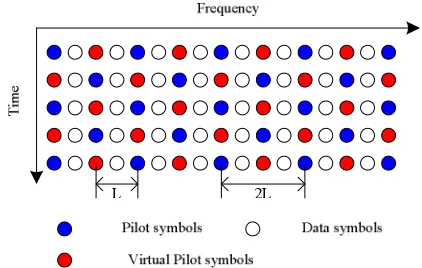
Assume that each OFDM symbol has N subcarriers where pilots occupy P subcarriers and virtual pilots su-perimposed with data samples also occupy P subcarriers. Figure 2 shows the proposed pilot arrangement as a platform, which is a special case but not loss of general-ity, where along frequency axis, the pilot spacing is 2L and the spacing between pilot and adjacent virtual pilot is L. From Figure 2, one can see that along time axis, the pilot spacing is 2 and the spacing between pilot and ad-jacent virtual pilot is 1. Also, by LS estimation, the CSI at pilot tones can be obtained by (1).

3.1. Time Interpolation at Virtual Pilot Tones

[image:3.595.317.528.80.214.2]

Denote the set of virtual tones by IPP. The CSI at vir-

Figure 2. The proposed pilot arrangement as a special plat-form, where the pilot tones in one OFDM symbol correspond to the virtual pilot tones in its adjacent OFDM symbol.

tual pilot tones is obtained by time interpolation. In this special pilot arrangement, since the virtual pilot tones at the mth symbol corresponds to the pilot tones at the

(

m−1 th

)

symbol, time replica at the virtual pilot tones in one symbol is to replicate the CSI at the pilot tones of its last symbol,

-1 ˆ _{( )} ˆ _{( ),}

m m PP

H k =H k k∈I . (10) On the other hand, if using time linear interpolation, we can get

-1 1

ˆ _{( )} ˆ _{( )}

ˆ _{( )} _,

2

m m

m PP

H k H k

H k = + + k∈I . (11)

3.2. Frequency Interpolation at Data Tones

Denote the set of data tones as ID. Using frequency

linear interpolation [20], the CSI at the whole OFDM symbol can be expressed as

(

)

(

)

ˆ _{( )} ˆ ₍ ₎

1 1 2 2

ˆ ₍ ₎

ˆ _{( )}

1 2 1 .

m m

m

L l l

H k H k L

L L

when k L P

H k l

H k

when k L P

−

 ₊ ₊



 ≤ ≤ + −

+ =   

 = + −



(12)

where (k+ ∈l) ID , k∈ ∪IP IPP, 1≤ ≤ −l L 1. Note

that the CSI for data tones located on the right side be-yond the

(

1+PL

)

th pilot/virtual pilot tone is decided by the edge interpolation.

4. Performance Analysis for the Special Case

[image:3.595.57.288.90.359.2]

(4)

4.1. MSE of Time Interpolators

For this special case, the MSE of time replica in (5) be-comes

{

2

}

2

1( ) .

R =Ek m− k +

ξ δ σ (13) On the other hand, the MSE of time linear interpola-tion in (8) becomes

2 2 1( ) ( )

. 2

m m

L k

k k

E  − − 

= _ _+

 

 

δ δ

ξ σ (14)

So, based on (13) and (14), the difference between ξR

and ξL can be obtained as follows,

{

}

2

2 2 1

1 ( ) ( ) 1 ( ) . 2 2 m m

R L k m k

k k

E ₋ k E  − − 

− = + −  

 

 

δ δ

ξ ξ δ σ

(15) And, from (15), one can conclude that 1) in a time- invariant frequency-selective channel, ξL is always

lower than ξR by 3 dB; in a time-variant frequency-

selective channel, the performance difference depends on the specific channel variation; 2) in most situations, as the general case in (9), ξR >ξL, i.e., time linear

inter-polation is better than time replica.

4.2. MSE of Channel Estimation

4.2.1. Time Replica

By LS estimation on pilot tones, time replica on virtual pilot tones and frequency interpolation on data tones, the corresponding MSE of channel estimation can be ex-pressed as

2 ,

LRL P R RF

P P N P

N N N

−

= + +

ξ ξ ξ ξ (16)

where ξP is the MSE of LS estimation and ξRF is the

MSE of frequency interpolation when using time replica at virtual pilot tones.

As an average of both odd and even OFDM symbols, except for the right side

(

L−1

)

tones using the edge interpolation, a half of other data tones with the index

(

k+ ∈l

)

ID have k∈IP while

(

k+ ∈L

)

IPP for

fre-quency linear interpolation; for the remaining data tones,

PP

k∈I while

(

k+ ∈l

)

IP for frequency linear

inter-polation. Hence, using (12), we can get ξRF in (17),

wheree_F(k l) L lH_m( )k l H_m(k L) H_m(k l)

L L

−

+ = + + − + ,

P PP

k I∈ ∪I , 1≤ ≤ +k 1 L

(

2P−2

)

, and e L P_F(1+ (2 -1) l+ ) (1 (2 -1)) - (1 (2 -1) )

m m

H L P H L P l

= + + + , are the

inher-ent errors by frequency interpolation, ξF is the inherent

MSE of frequency interpolation.

By substituting (17) into (16), ξLRL can be expressed

as the following (18),

{

}

{

}

2 , 2 , 1 2 , 1 2

ˆ ₍ _{) -} ₍ ₎

1 1

1 ( ) ( ) ( )

2 2

1 1

1 ( ) ( ) ( )

2 2

1

(1 (2 1) ) 2

2 1 1

1

6 2

RF k l m m

k l F m m

l F F

E H k l H k l

L L l l

E e k l W k k

N P L L

L l L l

E e k l W k k

N P L L

L

E e L P l

N P

L L

L N P

− − = + + =   −  −   ₋  _{+ +} ₊    ₋        −  −    + _ − _ _ + + + _ −     − + + − + = − −  − + _ − −  ξ δ δ ξ

{

}

2 2 1

2 1 1

1 ( ) ,

6 2 k m

L L

E k

L N P −

  −  −  + _ − _ −   σ δ (17)

(

)(

)

2

_{

2

_}

1 2

2 1 2 1

( ) . 6

LRL P R F

k m

P P N P

N N N

L N P L

E k NL − − = + + − − _{− + } _ + __ + __

ξ ξ ξ ξ

σ δ

(18)

4.2.2. Time Linear Interpolation

By LS estimation on pilot tones, time linear interpolation on virtual pilot tones and frequency interpolation on data tones, the MSE of channel estimation can be expressed as

2 ,

LLL P R LF

P P N P

N N N

−

= + +

ξ ξ ξ ξ (19)

where ξLF is the MSE of frequency interpolation when

using time linear interpolation at virtual pilot tones. Us-ing (12), ξLF can be obtained as shown in (20).

Substituting (20) into (19), ξLLL can be expressed as

the following (21),

{

}

{

}

2 , 2 1 , 2 1 , 2

ˆ ₍ _{) -} ₍ ₎

1 1 1 2 2 ( ) ( ) ( ) ( ) 2 1 1 1 2 2 ( ) ( ) ( ) ( ) 2 1

(1 (2 1) ) 2

LF k l m m

m m

k l F m

m m

k l F m

l F

E H k l H k l

L

N P

k k

L l l

E e k l W k

L L

L

N P

k k

l L l

E e k l W k

L L

L

E e L P l

(5)

2

2 1

2 1 1

1

6 2

( ) ( )

2 1 1

1 .

6 2 2

F

m m

k

L L

L N P

k k

L L

E

L N P

ξ σ

δ ₋ δ

−  − 

+ _ − _

−

 

 ₋ 

−  −   

+ _ − ₋ _  

 

 

(20)

(

)(

)

2

2 1

2

2 1 2 1

6

( ) ( ) . 2

LLL P R F

m m

k

P P N P

N N N

L N P L

NL

k k

E −

−

= + +

− − − +

+

 _ ₋ _

 +  

 _ _

 

ξ ξ ξ ξ

δ δ

σ

(21)

4.2.3. Comparison

Subtracting (21) from (18), the difference between ξLRL

and ξLLL can be obtained as

(

)(

)

{

}

2

2 ₁

1

2 1 2 1

2 6

( ) ( )

( ) .

2

LRL LLL

m m

k m k

L N P L

P P

N N NL

k k

E ₋ k E −

− − − +

 

− = +_ + _

 

 _ ₋ _

 

× − _ _

  

 

ξ ξ σ

δ δ

δ

(22) From (22), one can notice that

1) Since N >> P, 2 2

P

Nσ is negligible and the dif-ferential MSE using (22) is approximately independent with noise;

2) In a time-invariant frequency-selective channel,

LRL

ξ is approximately equal to ξLLL ; while in a

time-variant frequency-selective channel, the perform-ance comparison depends on the specific channel varia-tion;

3) Considering a real-valued channel variation, in low noise environment, when δm( )kδm−1( )k <0 and δm( )k >

1( )

m− k

δ , ξLRL<ξLLL;

4) ξLRL−ξLLL <ξR−ξL .

5. Numerical Results

The OFDM system under consideration is with N= 512 subcarriers, and 2L = 8 equispaced pilot tones in each symbol. The length of cyclic prefix is 32. The interpola-tion distances p = q = 1. The modulation is QPSK. The pilot tones are all 1. For 0≤ ≤j 63, in the odd OFDM symbols, the pilot is inserted at the

(

1 8+ j

)

th tone;

while in the even OFDM symbols, the pilot is inserted at the

(

5 8+ j

)

th tone. The six-ray multipath Rayleigh fading channel is considered. The average power delay profile is selected as

5 0 exp( )

l

l l

l

=

− =

∑

λ

λ , 0≤ ≤l 5. (23)

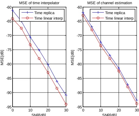
Figure 3 shows the MSE performance of time inter-polator and channel estimation in the time-invariant fre-quency-selective channel, where one can see that time linear interpolator generating less noise has a 3 dB lower MSE than time replica at the virtual pilot tones. However, for the corresponding channel estimation at the whole OFDM tones, time linear interpolator performs similarly to time replica due to a negligible noise.

Figure 4 shows the MSE performance in a time vary-ing channel where the parameters are Ek

{

δm−1( )k

}

0.001

= ,

{

}

6

1( ) 10

k m

Var δ ₋ k = − , Ek

{

δm( )k

}

= −0.002, and

{

}

6

( ) 10

k m

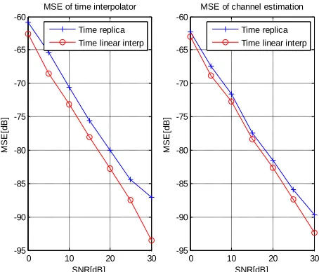
Var δ k = − , respectively. For interpolation at vir-tual pilot tones, when SNR≤25 dB, time linear inter-polator performs better than time replica due to better noise reduction; when SNR > 25dB, time replica, which guarantees a more accurate interpolation in a low noise environment, performs better than linear interpolator. While for the corresponding channel estimation, when

25

[image:5.595.66.291.77.260.2]

SNR≤ dB, time linear interpolator performs very similarly to time replica due to better noise reduction; when SNR > 25 dB, time replica also performs better than time linear interpolator.

Figure 5 shows the MSE performance in the time va-rying channel where the parameters are Ek

{

δm−1( )k

}

0 10 20 30 -95

-90 -85 -80 -75 -70 -65 -60

SNR[dB]

M

SE

[d

B]

MSE of time interpolator Time replica Time linear interp

0 10 20 30 -95

-90 -85 -80 -75 -70 -65 -60

SNR[dB]

M

SE

[d

B]

MSE of channel estimation Time replica Time linear interp

[image:5.595.311.538.493.683.2]

(6)

0 10 20 30 -90

-85 -80 -75 -70 -65 -60

SNR[dB]

M

SE

[d

B]

0 10 20 30 -90

-85 -80 -75 -70 -65 -60

SNR[dB]

M

SE

[d

B]

Figure 4. MSE of time interpolator and channel estimation in time-variant frequency-selective channel, where the ex-pectation is equal to Ek

{

δm−1( )k

}

=0.001, the variance is

equal to

{

}

6

1( ) 10

k m

Var δ ₋ k = − , the expectation Ek

{

δm( )k

}

0.002

= − , and variance

{

}

6 ( ) 10

k m

Var δ k = − , respectively, 0≤ ≤k 512.

0 10 20 30 -95

-90 -85 -80 -75 -70 -65 -60

SNR[dB]

M

S

E

[d

B]

0 10 20 30 -95

-90 -85 -80 -75 -70 -65 -60

SNR[dB]

M

S

E

[d

B]

Figure 5. MSE of time interpolator and channel estimation in time-variant frequency-selective channel, where the ex-pectation is equal to E_k

{

δ_m₋₁( )k

}

=0.001, the variance is equal to

{

}

6

1( ) 10

k m

Var δ ₋ k = − , the expectation E_k

{

δ_m( )k

}

0.002

= , and variance

{

}

6 ( ) 10

k m

Var δ k = − , respectively, 0≤ ≤k 512.

0.001

= , Vark

{

m1( )k

}

106

−

− =

δ , Ek

{

δm( )k

}

=0.002, and

{

}

6

( ) 10

k m

Var δ k = − , respectively. Time linear interpola-tor always performs better than time replica for both in-terpolation at the virtual pilot tones and the correspond-ing channel estimation at the entire tones.

6. Conclusions

Time replica and time linear interpolation were analyzed and compared, especially under our proposed pilot ar-rangement. The MSEs of both time interpolators were derived analytically for both interpolations at the virtual pilot tones and their corresponding channel estimation at the entire OFDM symbol. Numerical simulation results were demonstrated to reach an agreement with theoreti-cal analysis. From the given results, one can see that, in a time-invariant frequency-selective channel, when the interpolation distances p = q =1, time linear interpolator has a 3 dB lower MSE than replica at the virtual pilot tones while they provide a similar performance at the entire OFDM symbol. Moreover, one can also see that, in a time varying frequency-selective channel, time lin-ear interpolator outperforms time replica except the case, in a low noise environment, the CSI variation from the last OFDM symbol to the present symbol is negative to and has a smaller absolute value than that from the pre-sent symbol to the following symbol.

7. Acknowledgements

The author would like to thank all the anonymous re-viewers of the paper. The critical comments by all the reviewers have helped us to improve the quality of our paper.

8. References

[1] M. Engels, “Wireless OFDM Systems,” Kluwer Acade- mic Publishers, New York, 2002.

[2] L. Hanzo, “OFDM and MC-CDMA: a Primer,” John Wiley & Sons, Inc., Hoboken, 2006.

[3] H. Schulze, “Theory and Applications of OFDM and CDMA: Wideband Wireless Communications,” John Wiley & Sons, Inc., Hoboken, 2005.

[4] B. Bing, “Wireless Local Area Networks: The New Wire- Less Revolution,” Wiley-Interscience, New York, 2002.

[5] S. Methley, “Essentials of Wireless Mesh Networking,” Cambridge University Press, Cambridge, 2009.

[6] M. Ma, “Current Technology Developments of Wimax Systems,” Springer Verlag, New York, 2009.

[7] C. Pandana, Y. Sun and K. J. R. Liu, “Channel-Aware Priority Transmission Scheme Using Joint Channel Es- timation and Data Loading for OFDM Systems,”IEEE Transactions on Signal Processing, Vol. 53, No. 8, August 2005, pp. 3297-3310.

[image:6.595.62.284.77.265.2] [image:6.595.58.285.367.561.2]

(7)

[9] W. Zhang, X.-G. Xia and P. C. Ching, “Clustered Pilot Tones for Carrier Frequency Offset Estimation in OF- DM Systems,” IEEE Transactions on Wireless Communi- cations, Vol. 6, No. 1, 2007, pp. 101-109.

[10] X. D. Dong, W.-S. Lu and A. C. K. Soong, “Linear Inter- polation in Pilot Symbol Assisted Channel Estimation for OFDM,” IEEE Transactions on Wireless Communica- tions, Vol. 6, No. 5, May 2007, pp. 1910-1920.

[11] I. Budiarjo, I. Rashad and H. Nikookar, “On the Use of Virtual Pilots with Decision Directed Method in OFDM Based Cognitive Radio Channel Estimation Using 2x1-D Wiener Filter,” Proceedings of IEEE International Con- ference on Communications, Beijing, May 2008, pp. 703- 707.

[12] Q. F. Huang, M. Ghogho and S. Freear, “Pilot Design for MIMO OFDM Systems with Virtual Carriers,” IEEE Transactions on Signal Processing, Vol. 57, No 5, May 2009, pp. 2024-2029.

[13] J. H. Zhang, W. Zhou, H. Sun and G.Y. Liu, “A Novel Pilot Sequences Design for MIMO OFDM Systems with Virtual Subcarriers,”Proceedings of Asia-Pacific Confe-

rence on Communications, Perth,2007, pp. 501-504.

[14] R. Prasad, “OFDM for Wireless Communications Sys- tems,” Artech House, Boston,2004.

[15] A. R. S. Bahai, “Multi-Carrier Digital Communications,” Springer Verlag, New York, 2004.

[16] K. Jihyung, P. Jeongho and H. Daesik, “Performance Analysis of Channel Estimation in OFDM Systems,”

IEEE Signal Processing Letters, Vol. 12, No. 1, January 2005, pp. 60-62.

[17] P. Jeongho, K. Jihyung, P. Myonghee, K. Kyunbyoung, K. Changeon and H. Daesik, “Performance Analysis of Channel Estimation for OFDM Systems with Residual Timing Offset,” IEEE Transactions on Wireless Commu- nications, Vol. 5, No. 7, July 2006, pp. 1622-1625.

[18] H. Myeongsu, Y. Takki, K. Jihyung and K. Kyungchul,

“OFDM Channel Estimation With Jammed Pilot Detector Under Narrow-Band Jamming,” IEEE Transactions on Vehicular Technology, Vol. 57, No. 3, May 2008, pp. 1934-1939.

[19] A. Rosenzweig, Y. Steinberg and S. Shamai, “On Chann- Els with Partial Channel State Information at the Trans- mitter,”IEEE Transactions on Information Theory, Vol. 51, No. 5, May 2005, pp. 1817-1830.