R E S E A R C H
Open Access
A machine-learning phase classification
scheme for anomaly detection in signals with
periodic characteristics
Lia Ahrens
1*, Julian Ahrens
1and Hans D. Schotten
1,2Abstract
In this paper, we propose a novel machine-learning method for anomaly detection applicable to data with periodic characteristics where randomly varying period lengths are explicitly allowed. A multi-dimensional time series analysis is conducted by training a data-adapted classifier consisting of deep convolutional neural networks performing phase classification. The entire algorithm including data pre-processing, period detection, segmentation, and even dynamic adjustment of the neural networks is implemented for fully automatic execution. The proposed method is evaluated on three example datasets from the areas of cardiology, intrusion detection, and signal processing, presenting reasonable performance.
Keywords: Anomaly detection, Time series analysis, Phase classification, Machine learning, Convolutional neural networks
1 Introduction
Many real-world systems, both natural and anthro-pogenic, exhibit periodic behaviour. Monitoring such sys-tems necessarily produces periodic time series. In one particular instance of such a monitoring application, one is interested in automatically detecting changes in the periodically repeating pattern and thus anomalies in the systems operation. This type of anomaly detection occurs in a wide range of different fields and applications, be they medical, e.g. diagnosing diseases of the cardiovascular and respiratory systems, in industrial contexts, e.g. monitoring the operation of a transformer or rotating machinery, and in signal processing and communications. The pursued aims range from simple monitoring to intrusion detection and prevention.
Traditionally, anomaly detection is performed in the form of outlier detection in mathematical statistics. Numerous methods have been proposed, including but not limited to distance- and density-based techniques
[1, 2] and subspace- or submanifold-based techniques
[3–5]. Most of these approaches make no explicit use of
*Correspondence:[email protected]
1Deutsches Forschungszentrum für Künstliche Intelligenz, Trippstadter Straße 122, 67663 Kaiserslautern, Germany
Full list of author information is available at the end of the article
the concept of time and are therefore usually less suited for the analysis of time series. Methods making explicit use of the temporal structure include classical models from statistical time series analysis such as autoregressive–
moving average (ARMA) models [6], Kalman filters [7]
or more general hidden Markov models [8], and
rolling-window distance-based methods such as matrix profiles [9]. Distance analysing methods are effective for clean data but not robust against noise, whereas distribution-based methods from mathematical statistics are still powerful in the presence of noise, requiring data-specific parameteri-sation. In the past few years, non-linear methods, such as different types of recurrent neural networks (RNNs) and in particular long short-term memory (LSTM) networks
have also come into use [10, 11]. Many of these
meth-ods are difficult to train [12–14] or need large amounts of data in order to achieve reasonable performance while avoiding overfitting. On the other hand, in recent years, convolutional neural networks (CNNs) have gained pop-ularity in image processing [15, 16] where they are used mainly for classification tasks. The same principles that are responsible for the success of CNNs in image process-ing carry over to other types of signal processprocess-ing when the number of dimensions of the convolutional kernels is changed accordingly. Most of the work using recurrent or
convolutional networks for time series analysis focuses on forecasting or detecting certain patterns explicitly known at training time. On these tasks, convolutional networks have recently been shown to outperform the previously state of the art LSTMs [17].
In this paper, we consider data with periodic character-istics and design a machine-learning algorithm for time series analysis, in particular anomaly detection, apply-ing convolutional neural nets in a manner which, to the best of the authors’ knowledge, has not been proposed previously. In contrast to existing methods and inspired by machine-learning methods for image processing, we employ a convolutional net acting not as a predictor or estimator but as a classifier whose classes indicate phase, i.e. the relative location in time. We also integrate gen-eral procedures for data pre-processing and automated phase reclustering so that no manual action is required in between.
Our algorithm is tested on three datasets: a cardiology dataset (ECG database) [18], an industrial network dataset for cyber attack research (SCADA dataset) [19], and a syn-thetic waveform dataset described in detail in Section4.3. It turns out that, to a certain extent, our method is robust against unclean data, and the related neural networks do not show high sensitivity to the hyperparameters and are relatively easy to train.
The remainder of the paper is organised as follows.
In Section 2, we specify the types of anomaly
detec-tion considered in this paper, comment on tradidetec-tional methods, and introduce the concept of our solution.
In Section 3, our general approach to the considered
anomaly detection problems is described in detail, includ-ing data pre-processinclud-ing, mathematical basis of convo-lutional neural networks, and training algorithm. In
Section4, our method is fine-tuned for the three
afore-mentioned example datasets and in Section5the
empir-ical results are evaluated. In Appendix A, dealing with
the issue of randomly varying period length which shows up in many real-world applications such as in the ECG
data (Section 4.1) and synthetic waves (Section4.3), an
auxiliary period detection scheme is designed based on
classical principles of signal processing. In Appendix B,
we perform some comparisons with other methods for anomaly detection in order to further highlight the advan-tage of using a convolutional neural network in the proposed manner.
2 Preliminaries
In preparation for the detailed description of our machine-learning phase classification scheme given in Section3, in this section, we clarify the tasks of anomaly detection in time series with periodic characteristics, dis-cuss some common methods, and outline the essential ideas of our approach.
2.1 Context of this work
In general, a time series {Xt}t=0,1,2,... (i.e. a tempo-ral sequence of observations X0,X1,X2,. . ., also termed signal) is said to exhibit periodic behaviour with
period length s if similarities occur after every s time
units, i.e. observations that are s time units apart,
Xt0,Xt0+s,Xt0+2s,. . .for anyt0, are similar.
Periodic signals occur naturally in a wide range of appli-cations and in a large number of fields such as audio processing, vibration analysis, biomedical engineering, climatology, and economic time series analysis. Often-times, one wishes to monitor the behaviour of such a sys-tem. In particular, a common task when observing a signal is that of anomaly detection, i.e. the detection of devia-tions from a certain normal mode of operation. This has a variety of applications such as disease diagnosis, network security, and fraud recognition in bank transactions.
The general approach to anomaly detection is to relate a mathematical model (parametric or non-parametric) to the normal behaviour of the underlying system based on historic observations (training data) and set a confidence region for data of normal type; applying the data-adapted model to the ongoing observations (test data), whether the output lies within or outside the pre-defined confidence region decides if the corresponding input observation is considered normal or abnormal, respectively.
As with most naturally occurring signals, many of the aforementioned signals do not satisfy the exact mathe-matical definition of periodicity. Instead, they exhibit a property which is referred to as quasiperiodicity which basically means that the signal does not exactly repeat itself, but has deviations both in its values and in the length of the actual periods. This behaviour is very common for instance in biological or climatological sys-tems. As a consequence for the task of anomaly detec-tion, a sophisticated mathematical model is required to capture the essence of the diverse and noise-corrupted signals.
2.2 Tasks of anomaly detection
Mathematically, the approach to anomaly detection pro-posed in this paper applies to the following two types of problems:
Type A The historic observations of normal type (training data) are made up of various signals
ι ∈ I, share certain common
normal-type-characterising features, but differ in their values and exhibit periodic characteristics with individual
period length s(ι) which may also fluctuate over
Type B The historic observations of normal type (train-ing data) are made up of consecutive s(train-ingle data points X0,X1,. . .,XN−1 which jointly form a time series {Xt}t=0,...,N−1. The occurrence of the data points X0,. . .,XN−1 follows certain normal-type-characterising patterns, which is reflected in the corresponding time series{Xt}t=0,...,N−1as seasonal
effects associated with period lengthswheresmay
randomly vary over time. The task of anomaly detec-tion in such a setting consists in specifying
seg-ments of ongoing observations {Xt}t≥N which are
abnormal.
Problems of type A arise from areas such as disease diag-nosis, climatology, and vibration analysis, whereas prob-lems of type B are often addressed in the security sector and building monitoring systems within the framework of signal processing. In general, establishing an adequate mathematical model for the normal behaviour of a sys-tem requires a proper amount of training data. In our
experiments in Section4, our approach to the considered
problems is applied to a cardiology dataset for detecting
heart disease (cf. ECG database [18]) as an example of
problems of type A, a relatively small industry dataset in
the context of network security (cf. SCADA dataset [19])
as an example of problems of type B, and a more exten-sive synthetic waveform dataset injected with a variety of
noise and anomalies (cf. Section4.3) again as an
exam-ple of problems of type B. The experimental results are provided in Section5.
From a mathematical perspective, problems of type A are more challenging than those of type B. In the setting of type A, a considerably complex mathematical model is needed for capturing diverse variations of the normal behaviour across a variety of training signals, whereas in the setting of type B, the required mathematical model for the normal behavior is to be fitted to a single training time series. Many traditional methods for anomaly detection in periodic signals may find direct applications to problems of type B but fail to be applicable to problems of type A. This will be further discussed in the subsequent section.
2.3 On common methods
Let us comment on the adequacy of some traditional methods for detecting anomalies in periodic signals in our context.
2.3.1 Distance-analysing methods
The most straightforward treatment of seasonal data goes back to cross-correlation analysis, e.g. matrix profiles [9]. The basic idea therein is to apply a rolling window and define a Euclidean-type metric which measures the dis-tance of consecutive values within the rolling window at different locations of the underlying time series from one another or from a fixed reference sequence (e.g. a
mean window consisting of seasonal means); data points exhibiting large distance from the reference value are considered abnormal.
In general, distance-analysing approaches are not resis-tant against noise and fail to capture complex structures
in the data. In the Appendix B, we evaluate a simple
distance-based self-similarity approach in “Self-similarity approach” section. We also provide a distance-based ver-sion of our phase classification scheme (without
artifi-cial neural networks) for comparison in “Distance-based
phase classification” section.
2.3.2 ARIMA methodology and Kalman filtering
A more sophisticated class of methods arises from mathematical statistics, e.g. autoregressive integrated
moving average (ARIMA) methodology, methods
based on structural component time series models or more general Kalman filtering (based on the linear case of the general state-space model or hidden Markov model), cf. [20,21] for detailed description of the corresponding mathematical models. These approaches can be directly
applied to problems of type B described in Section2.2and
are based on relating a stochastic model with parameters = θ1,. . .,θrto the training part{Xt}t
=0,1,...,N−1 of
the observed time series{Xt}t so as to make short-term
(usually one-step ahead) forecasts, i.e. to estimate the conditional expectation E[Xt+t | Xt,Xt−1,. . .;] by
ˆ
Xt+t for all t (in particular for t + t ≥ N), which
basically relies on calculating the maximum likelihood
estimateˆ of the parameters , making use of available
observations. Setting a threshold value δ, if the actual
observationXt0varies enough from the forecast valueXˆt0
in the sense that|Xt0 − ˆXt0| > δ, then the data pointXt0
observed at timet0is considered abnormal.
pre-processing, e.g. logarithmising, power transforma-tion, and differencing) and a data-adaptive
hyperparam-eter choice (i.e. the design of the paramhyperparam-eter set =
θ1,. . .,θr, in particular the number of parameters r) which relies on inspection of the autocorrelogram and partial autocorrelogram. Each ARIMA model has an equivalent linear state-space model representation allow-ing Kalman filterallow-ing to be employed for forecastallow-ing.
The ARIMA approach and Kalman filtering are pow-erful tools in many applications and in particular in the presence of noise, provided that the hyperparameter choice is reasonable. However, being the most technically manageable segment of the general state-space models, linear models lack complexity and therefore do not always deliver a feasible approximation for real-world applica-tions. In addition, the associated data-adapted model selection including data pre-processing requires specific expert knowledge and is therefore difficult to imple-ment for fully automatic execution as in our machine-learning framework. Furthermore, considering problems
of type A described in Section 2.2, it is unclear how
to choose a general representative time series Xt∗t in which the diverse variations arising from the
individ-ual training signals X(ι)t t | ι ∈ I are incorporated
so that the model fitted to Xt∗t applies to all normal signals.
2.3.3 Long short-term memory units
Long short-term memory units (LSTMs) are a special type of recurrent neural network (RNN). As such, the LSTM reads the input time series sequentially, transform-ing at each point in time the input data into a hidden state which is a non-linear function of the current input and the hidden state one time step earlier. The advan-tage of LSTMs over most other types of RNN is that the dependency of the current on the previous hidden state is designed in such a way that the LSTM obtains the abil-ity to keep (parts of ) its hidden state over a larger number of time steps than is possible with other RNN archi-tectures, i.e. LSTMs are able to “memorise” values from the past.
Applying LSTMs to prediction tasks for the purpose of anomaly detection works in a similar manner to the appli-cation of statistical methods described in the beginning
of Section 2.3.2. The main differences are that LSTMs
allow for non-linear parameterisation and have the poten-tial to support a much larger number of parameters which are not estimated directly but instead are randomly ini-tialised at first and then optimised during training (learnt) to obtain the desired predictor. The complexity of the LSTMs allows them to ingest characteristics of rich and varied training data such as those from large training data sets of type A as described in Section2.2through the pro-cess of training with a stochastic gradient descent (SGD)
type algorithm. The training set is processed repeatedly and the parameters of the LSTM are adjusted to opti-mise the quality of the forecast across the entire training dataset.
Technically, the main drawback of LSTMs is the fact that they are fundamentally still RNNs and hence also suffer from some of the difficulties typical for training this class of artificial neural network such as exploding gradients and a high potential for overfitting.
As a general drawback of using one-step ahead pre-diction for anomaly detection in time series, if the time series is very complex and exhibits regions in which it is difficult to make precise forecasts, such as when analysing periodic signals containing steep edges or spikes whose positions or values vary randomly over time, reli-ably estimating the values in these regions can actually be impossible for any type of one-step ahead prediction. It is thus difficult to derive an anomaly detector from such a predictor as the estimated values can have a large distance to the actual ones and thus show up as false
pos-itives. In Appendix Bsection, this is illustrated in more
detail by training and evaluating an LSTM on the ECG database.
2.4 Concept of this paper
Let us now introduce the concept of our machine-learning phase classification approach to the problems specified in Section2.2.
2.4.1 Motivation of using convolutional neural networks for phase classification
Convolutional neural networks (CNNs) are a specific architecture of feed-forward neural networks. When com-pared to a fully connected neural network, convolu-tional neural networks need fewer parameters. Hence, they do not require as large a training dataset and are less prone to overfitting. CNNs make explicit use of the temporal or spatial structure of the input signal; the sig-nal is asig-nalysed locally (local receptive fields) and in a shift invariant manner (translation invariance). Investiga-tions on the internal representaInvestiga-tions present throughout the layers of CNNs show a high tolerance to noise of various kinds.
Like LSTMs, compared to statistical methods, CNNs have the advantage that, through the use of multiple chan-nels and non-linearities, they provide enough flexibility to capture intricate structures of analysed signals and are able to find representations for large and varied datasets. They are however easier to train than RNNs, as they suffer less from the vanishing and exploding gradient problems. The capability of a CNN of being able to process high amounts of complexity has been analysed in the field of
image processing, where it was shown [22] that the
patterns ranging from simple edges to things as complex as faces.
While CNNs can be used to make forecasts in time series, they particularly excel at classification of spatial or temporal data. Since the main problem of the LSTM-based approach to anomaly detection in time series out-lined above is the general unfeasability of using one-step ahead forecasts, we capitalise on the strength of CNNs in classification tasks and devise a new type of anomaly detection scheme relying on phase classification instead of one-step ahead forecasting. More details on the properties
and operation of CNNs are given in Section3.2.
2.4.2 Phase classification and anomaly detection
Motivated by the advantages of convolutional neural net-works in classification tasks when dealing with spatial or temporal data, the machine-learning approach proposed in this paper is based on the following key ideas:
1. Conducting multi-dimensional time series analysis by means of multi-channel deep convolutional neural networks, where each channel in the input layer corresponds to a single feature (dimension) of the considered time series
2. Identifying phases or, equivalently, relative locations (order of occurrence) of subpatterns from time series with periodic characteristics by means of training data-adapted classifiers so that subpatterns over different periods of the underlying time series are properly separated into a certain amount of classes
To be more specific, considering a seasonal time series {Xt}t with period begins (e.g. time of local peak values) {τk}k, for a pre-determined initial number of classes n0,
sampling from the original signal n0 overlapping
seg-ments per period with asliding window of length T, each
subpatternXt(m)
t=0,...,T−1with
Xt(m):=Xτk+(τk+1−τk)(mmodn0)/n0+t, k= m/n0,
m∈N, is assigned to the class labelledmmodn0. For seasonal data, subpatterns sampled from the time series occur repeatedly and in fixed order within each sin-gle period. A successfully trained classifier outputs the correct class indicating the phase or, equivalently, the rela-tive location in time (i.e. time distance between subpattern and period begin) of the input subpattern. Abnormal dat-apoints in an input pattern are expected to cause false classification results and therefore to be identified as anomalies, which yields a direct solution to problems of
type B described in Section2.2. For problems of type A
described in Section 2.2, setting a minimum expected
classification accuracy (threshold value) and evaluating the classification accuracy of each test signal over a
cer-tain number of periods (which is denoted by K in the
sequel), those signals that fail to achieve this minimum are considered abnormal.
In order to optimise the classification accuracy of nor-mal data and hence prevent false-positive anonor-maly detec-tion results, we carry out a dynamic reclustering which cancels confusing classes, i.e. subpatterns within a period of the signal that are similar enough to one another are merged into one class. This reclustering procedure along
with the optimisation of the stride length t := s/n0
(i.e. time distance between the segments to be classified) is implemented as a dynamic model selection scheme inte-grated in our training algorithm. In addition, we design an auxiliary period detection scheme which is employed in case of a randomly varying period lengths.
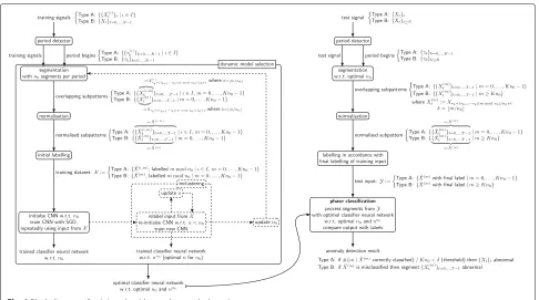
The block diagram in Fig. 1 outlines the major steps
of our training algorithm and anomaly detection scheme where the steps marked by dashed lines are conditioned by some model-adequacy monitoring criteria which are described in the subsequent section.
3 Method
In this section, we present the general procedure of our phase classification scheme in detail and provide some guidelines for the hyperparameter choice.
3.1 Data pre-processing
Prior to being fed into the classifier neural nets, all input signals (including training, validation, and test data) are processed by a period detector, cut into overlapping seg-ments by a sliding window, and subsequently normalised, where the segmentation and normalisation depend on the initial number of classesn0.
3.1.1 Period detection
In general, the seasonal effects of a time series can be recognised by examining the autocorrelogram (cf. [20, 2.1.4]) or periodogram (cf. [20, 2.2.1]). In many cases, the period lengthsis fixed and known. In case of a fluctu-atings(cf. e.g. data from cardiology), an auxiliary period
detector is designed in Appendix A, capturing the time
of local extremum values (considered as period begins in our setting){τk}k within individual periods and using cross-correlations in order to achieve robust period detec-tion. Note that in our setting for randomly varying period
lengths, the stride lengtht = s/n0 while segmenting
the signal varies proportionally tos so that the number
of overlapping segments from each period is fixed and equal ton0.
3.1.2 Sliding window
The classification accuracy of our approach turns out not to be highly sensitive to the length of the sliding
win-dowT. In the context of anomaly detection, the value of
T should be kept relatively small (e.g. less than or equal
Fig. 1Block diagram of training algorithm and anomaly detection
the abnormal data points on the time series. We use a
window size ofT = 3s/n0(approximately three times
the stride length) where srefers to the average value of
s (recall that in general s may vary over time).
Empiri-cally, this has proven to be adequate for our purpose. Note that the length of the sliding window remains constant
even in the case of randomly varying period lengths, the
varying stride length merely affects the amount of overlap between adjacent sliding windows.
3.1.3 Normalisation
In order to remove trend components and avoid skewed results due to dominating extreme values, the samples within the sliding window are normalised by adjusting the local mean and variance, that is, each time considering a d-dimensional time series {Xt}t = Xtiit=0,...d−1 with period begins{τk}k to be processed by a classifier neural network corresponding to initial number of classesn0, for
i=0,. . .,d−1 andm∈N, the vector
˜
Xti,(m)
t=0,...,T−1is
fed into channeliof the convolutional neural net, where
˜
Xti,(m):= X
i,(m)
t −μi,(m)
σi,(m) for t=0,. . .,T−1 with
Xti,(m):=Xiτ
k+(τk+1−τk)(mmodn0)/n0+t, k= m/n0,
μi,(m):= 1
T
T−1
t=0
Xti,(m),
σi,(m):=
1
T
T−1
t=0
Xti,(m)−μi,(m)2.
For the training and validation data, each subpattern ˜
X(m) := { ˜Xt(m)}t=0,...,T−1is initially labelledmmodn0. If reclustering occurs during the training so that the training and validation inputs are relabelled (cf. Section3.3.3for more details), then the test data are labelled in accordance with the final labelling of the training and validation data.
3.2 Convolutional neural networks
The core of our phase classifier is a convolutional neural network (CNN). CNNs are a special type of feedforward neural network, which exploit structures of space or time by sharing many of the weights among different neu-rons. We provide a short description of the mathematical basis of a convolutional neural network. For more detail on the subject, we refer the reader to the literature, e.g. [23, Ch. 9].
Basically, a feedforward neural network is a function
f:RN(0)×RP−→Rn, mapping an input vectorx∈RN(0) to an output vectory = f(x,p) ∈ Rn, using a vector of
parametersp ∈ RP to adapt the mapping. When acting
as a classifier, n is the number of classes and the
f(x,p)=f(L−1)· · ·f(0)x,p(0)· · ·,p(L−1)
whereLis the number of layers and forl = 0,. . .,L−1 the functionsf(l):RN(l)×RP(l) −→RN(l+1) are the trans-formations performed by each of the single layers and the vectorsp(l) ∈ RP(l) are again parameter vectors used to
adapt the mapping and given as subvectors ofp. For ease
of notation, let us denote the input to the functionf(l)by
x(l), starting withx(0) = xand the output of the function
f(l)byx(l+1), ending withx(L)=y.
In the most simple feedforward neural networks, each of the transformationsf(l)is given by a multiplication with a matrixa(l) ∈ RN(l)×N(l+1) called theweight matrix fol-lowed by an addition of a vectorb(l) ∈ RN(l+1) called the
bias vectorfollowed by the application of some non-linear
functiong: R−→Rcalled theactivation functionto each
of the components of the resulting vector, i.e.
x(l+1)=f(l)(x(l),p(l)) the components of the parameter vectorp(l). This is called afully connectedlayer.
In the case of a one-dimensionalconvolutional layer, the affine transformationx(l) −→x(l)·a(l)+b(l)is replaced with a more restrictive kind of affine transformation, the so-called batched convolution. For this, the vectorx(l) =
x(il)
i<N(l) is reindexed to form a two-dimensional array
x(i,tl)
i<M(l),t<T(l) withM(l)·T(l) = N(l), and we say that
the sequencex(i,tl)
t<T(l)is fed into theithchannelof the
convolutional layerl.1Similarly, the parameter vectorp(l)
is distributed not into a matrixa(l)and a vectorb(l), but into a matrix of vectors k(i,j,sl)
i<M(l),j<M(l+1),s<S(l) called the convolution kernelsand a vectorb(l) ∈ RM(l+1). The operation performed by the functionf(l)is now given by
x(l+1) In many convolutional networks, the input vectors
x(i,tl)
t<T(l) are extended (padded) by additional zero
entries prior to being convolved. When padding with exactlyS(l)−1 zeros, the output vectors are of the same size as the input vectors. If furthermore the padding is performed symmetrically, i.e. if S(l)−1/2 zeros are added to both ends of the signal, this is referred to as ‘SAME’-padding.
We also use a type of layer called max pooling layer
between two convolutional layers. The transfer function
f(l):RM(l)×T(l) −→RM(l+1)×T(l+1)of this layer is given by
where R(l) is a positive integer called the pool size
and we have the constraints M(l+1) = M(l) and
T(l+1) = T(l)/R(l). Note that max pooling layers have no adjustable parametersp(l).
In our networks, we employ both convolutional and reg-ular fully connected layers. We apply SAME-padding in all convolutional layers and use the hyperbolic tangent
(tanh) as activation functiongthroughout the entire
net-work, which is a common choice in feedforward neural networks.
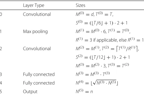
The exact layout of the convolutional network used for our task is displayed in Table1. Hered,T, andndenote the dimension of the input time series, the sliding window size, and the current number of classes, respectively. The layer and kernel sizes are chosen to best adapt to varying input time series dimensions, sliding window sizes, and numbers of classes. In the convolutional layers, the num-ber of channels is increased first by a factor of 6, then by a factor of 3. Such increases are common in convolutional neural networks and allow the layers to capture different aspects of the incoming signal such as edges and more complex patterns.
Table 1Layers of classifier neural network
The method, by which the parameter vector p is adjusted and the network adapts, is the minimisation of a
functionh: Rn −→Rapplied to the output of the neural
network, called theloss function. Since we are classifying
phases, to each training inputx(and hence to each output
y), there corresponds a labelz∈ {0,. . .,n−1}. In our case, we use the cross entropy loss function, which is given by
h(y,z)= −wzlog
expyz
M−1
j=0 expyj
where wz denotes a weight by which the losses of each
class are scaled. The weights are statically determined and are in our case chosen to be proportional to the inverse of the number of training examples for each class in order to counteract bias caused by unbalanced classes.
3.3 Training algorithm
The neural networks in our algorithm are trained by the ADAM training algorithm which is a refined version of stochastic gradient descent (SGD). In SGD, the average loss for a setXbatchcontaining pairs of training inputsx
and corresponding labelszis minimised by changing the
randomly initialised parameterspof the neural network
according to the update rule
p←p− γ
#Xbatch
(x,z)∈Xbatch
∇ph(f(x,p),z)
where γ is a tuning hyperparameter called the learning
rateand∇p is the gradient operator with respect to the
vector of parameters p. This minimises the average of
the loss valuesh(f(x,p),z). The gradient∇ph(f(x,p),z)is computed in an efficient manner via reverse-mode auto differentiation which is basically an application of the chain rule. This is also known as the backpropagation algorithm and more details on the process can be found in the literature, e.g. [23, Ch. 4]. The setXbatchis called a
mini-batchand is taken to be a subset of the set of all
avail-able training inputsX. The update steps are performed
with changing disjoint mini-batches until the entire
train-ing datasetX is exhausted. Each pass through the entire
set of available training data is referred to as anepoch. To enhance the training process (cf. [24]), for rich datasets, we change the size of the mini-batches during training, later epochs use larger mini-batch sizes. The adaptive adjustments performed by the ADAM algorithm detailed in [25] provide further enhancements to this process.
In contrast to usual classifiers, our algorithm encapsu-lates the gradient descent algorithm in a decision process
monitoring the necessity of dynamic reclustering which
aims to optimise the classification accuracy. The complete
algorithm is given in Algorithm 1 (cf. also Fig.1), the single steps are described in more detail in the remainder of this section.
Each time having initialised the neural network for separating the currently considered classes, the gradi-ent descgradi-ent optimiser is run until a training-progress-monitoring stop criterion is fulfilled (cf.training stop cri-terionin Section3.3.2for more details). The classification ability of the underlying neural net is evaluated by means
of the so-called confusion matrices (cf. Section 3.3.1)
throughout the entire training. If at the end of training all classes are evaluated with sufficient accuracy (cf. reclus-tering stop criterion in Section3.3.2), the trained neural net is stored; otherwise, a relabelling procedure
accord-ing to the overall confusion matrix is conducted where
net is re-initialised with respect to the updated classes (cf. Section3.3.3). Among all stored neural nets, the ulti-mate classifier is chosen as the one having the maximum number of output classes (cf. Section3.3.4).
In the subsequent subsections, the aforementioned reclustering process and stop criteria are described in detail.
3.3.1 Confusion matrix
In order to track the progression of classification
accu-racy during training, we record the confusion matrix
evaluated on the training data after each epoch. For a
current number of classesnand existing classes labelled
as 0,. . .,n−1, the confusion matrix evaluated after the
to the number of training inputs labelled asi and
pre-dicted by the neural net during thekth training epoch as
classj,k≥0.
During the experimentation, we observe that classes which are easily distinguishable can already be separated after very few training iterations, whereas classes sharing more similarity perform significantly worse in the begin-ning and also show a slower increase of evaluation accu-racy during training. Taking into account that the evalu-ated value of the loss function commonly follows a convex decreasing trend throughout the entire training, the above observation motivates us to assess the separation ability of the underlying neural net during training by weight-ing the confusion matrix with the respective contribution
to the training progress and to introduce theoverall
con-fusion matrixdenoted byV(n) := Vij,(n) classes, the number of training epochs that are performed until the training stop criterion (cf. Section3.3.2) is
satis-fied, and the average training loss during thekth epoch,
respectively.
In our setting, the confusion matrices serve as the key objects of the decision criteria for our dynamic reclus-tering (cf. Sections3.3.2and3.3.3). The definition of the
overall confusion matrix in terms of (1) by taking the
weighted average throughout the entire training and
drop-ping the values from the initial epoch (k = 0) aims to
mitigate the random effect of the initialisation of the neu-ral network. Empirically, this yields robust reclustering results during different test runs for fixedn0.
3.3.2 Stop criteria
The criteria for stopping the loops are related to param-eterised effectiveness and accuracy requirements in the following manner:
Training stop criterion We monitor the training progress by evaluating the average loss of vali-dation data over each training epoch. For each (re-)initialised neural network, training is stopped if no improvement in the average validation loss during the latest four epochs can be observed. Reclustering stop criterion Allowing a maximum
per-class margin of errorα∈[0, 1), the reclustering
pro-ber of classes, numpro-ber of epochs for training the related network (i.e. until the training stop criterion is fulfilled), and the respective confusion matrix eval-uated at the end of training (recall the definition in Section3.3.1), respectively.
By definition of the confusion matrix in Section3.3.1,
for k = E(n) − 1 and each i = 0,. . .,n − 1, the
diagonal element Vkii,(n) divided by the respective row sumnj=−01Vkij,(n) of the confusion matrix is the share of correctly classified training inputs in all training inputs
labelled asievaluated during the last epoch while
train-ing the classifier neural network withnexisting classes.
Therefore, for a pre-defined margin of error α∈[0, 1),
the above reclustering stop criterion requires that at the end of training the corresponding classifier neural net-work should correctly classify the training inputs of each existing class at least at the rate of 1−α.
3.3.3 Reclustering
As long as the reclustering stop criterion is not fulfilled, the subsequent reclustering procedure is considered nec-essary.
For a current number of classesnand existing classes
j◦:= arg max j=0,...,n−1
j=i◦
Vi◦j,(n)
respectively (recall the definition ofV(n)in (1)). The class labelled asi◦ is merged into classj◦. Furthermore, since we always assume the labels to be consecutive, the
train-ing and validation inputs with the largest labeln−1 are
assigned the label of the dropped classi◦.
Each time after relabelling, the weights corresponding to the remaining classes in the cost function are adjusted to be again inversely proportional to the current shares of the classes in order to warrant a well-balanced training of the updated classifier and the neural net is re-initialised.
3.3.4 Final number of classes
In the context of anomaly detection, we are dealing with the trade-off between optimising the classification accu-racy of normal data preventing false positives (i.e. to cancel confusing classes) and maintaining the ability of misclassifying abnormal data for the sake of anomaly detection (i.e. to still retain sufficiently many classes char-acterising different phases within a period). Keeping this in mind, the final number of classes determining the ulti-mate classifier neural network is selected in the following manner:
Given a maximum allowed number of classes n∗0 with
n∗0an even numbern∗0 >3, the starting initial number of classes is set ton0:=n∗0. Each time for an updated initial number of classesn0, the relabelling procedure described in Section 3.3.3is run at most(n0−3)-times (i.e. with at least 3 remaining classes). If the reclustering stop crite-rion is fulfilled after relabellingnn0-times, thecandidate
final number of classes related to n0 is set to nn0 :=
n0 −nn0 and the corresponding neural net is stored.
If maxn
0=n∗0,...,n0n
n0 ≥ n
0−2, the updating processes of
n0 is finished; otherwise n0 is reduced by 2. The
over-all final number of classesrefers to the maximum ofnn0
taken along the entire path ofn0, i.e. maxn0=n∗0,...,4nn
0and
the final classifier neural network is the one stored when this overall maximum was achieved. If this maximum was achieved more than once, we choose the neural network
corresponding to the highest n0 such that nn0 achieved
this maximum. This is because a high value ofn0
corre-sponds to a narrow sliding window (cf. Section3.1.2) and
hence maximises the sensitivity of the anomaly detector. If in the end no suitable network has been stored, we
increaseαand rerun the algorithm.
Finally, it is worth mentioning that once all the hyperparameters are determined, the whole training
algorithm introduced above, including data
pre-processing and dynamic reclustering, is implemented in a machine-learning manner so that the classification
and anomaly detection process can be accomplished fully automatically.
3.4 Anomaly detection
Once training is finished and in particular when the ulti-mate classifier neural network determined by the model selection process turns out to use initial number of classesn0and final number of classesnn0, each test sig-nal is pre-processed following the procedure described in
Section 3.1 with respect to n0, labelled with respect to
nn0 in accordance with the training and validation data
(recall the relabelling step along with the dynamic
reclus-tering described in Section3.3.3), and then processed by
the trained ultimate classifier neural network.
For problems of type A described in Section2.2, a
min-imum expected per-signal average classification accuracy
δ (threshold value) should be set depending on
individ-ual needs. For instance, δ could be determined on the
basis of classification accuracy on validation data. For each
test signal {Xt}t recorded over K periods of time with
period begins {τk}k=0,...,K−1, if the normalised segments ˜
X(m),m=0,. . .,Kn0−1 (recall Section3.1.3), processed by the ultimate classifier neural net are evaluated with an average classification accuracy rate less thanδ, i.e. if #{m | ˜X(m)correctly classified}/Kn0 < δ, then the signal {Xt}tis considered abnormal.
Considering problems of type B described in
Section 2.2, if a normalised segment X˜t(m)t=0,...,T−1
(recall Section 3.1.3) of the test signal {Xt}t≥N is mis-classified by the ultimate classifier neural net, then the original segmentXt(m)t=0,...,T−1with
Xt(m)=Xτk+(τk+1−τk)(mmodn0)/n0+t, k= m/n0
is considered abnormal.
4 Experiments
In this section, we apply our machine-learning
algo-rithm proposed in Section 3 to three example datasets
choosing from the domains of cardiology, industry, and signal processing, aiming to show the feasibility of the method in a range of applications. The cardiology dataset is the most complex and challenging dataset
represent-ing problems of type A described in Section 2.2, as the
4.1 Cardiology dataset
The PTB Diagnostic ECG Database is a database cre-ated by the Physikalisch-Technische Bundesanstalt (PTB) consisting of 549 electrocardiogram (ECG) recordings gathered from 290 subjects aged 18 to 87. The ECGs were recorded using a non-commercial PTB prototype recorder, the specifications of which can be found on the database website2. The dataset is part of PhysioNet [26] and is further described in [18].
4.1.1 Input data
We use 3/5 and 1/5 of the measurements from healthy
patients for training and validation, respectively. The trained classifier is tested on the remainder of the data from healthy patients and data from all ill patients.
Due to the large data volume, we manually resample the input data to a sample rate of 50 samples per sec-ond instead of the original 1000 before feeding it into the neural network (i.e. the actual time unit applied in our
training amounts to 1 time unit = 20 ms). This
opera-tion is not strictly necessary, but it speeds up the training process. Also, we only use the first 60 periods of each recording during training and for testing. We train our classifier with resampled time series from healthy patients and use the data coming from all 12 conventional leads and 3 Frank leads (cf. [27]) for the ECG diagnostic, result-ing in a convolutional neural net with 15 channels on the input layer.
4.1.2 Period detection
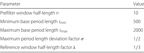
The first challenge when analysing ECG data consists in detecting the randomly varying periods of individ-ual patients, for which we design a period detector. This detector is described in greater detail in AppendixA. The detector has a number of parameters which need to be adjusted to the dataset, the actual values used here are given in Table2. For this dataset, the entire time series for feature ‘i’ is used as both the reference and input time series to the period detector. However, in order to ensure the requirement that no trend component exists in the signal, the first difference of the signal is used instead of the raw signal. In order to adjust for the
off-sets thus introduced at peak detection, between steps4
and 5 described in Appendix A, the reference window
Table 2Parameters for period detector on ECG database
Parameter Value
Prefilter window half-lengthn 10
Minimum base period lengthsmin 500
Maximum base period lengthsmax 2000
Maximum period length deviation factorσ 1/2
Reference window half-length factorλ 1/3
is adjusted to be precisely centred on the correspond-ing peak in the original (smoothed but not differentiated) signal, i.e. its midpointTk0is changed to
arg max Tk0−10≤t≤Tk0+10
Xt.
The maximum allowed adjustment of 10 has empirically been found to yield satisfactory results.
The median of all observed period lengths
approxi-mately amounts tos=700 ms=35 time units.
4.1.3 Hyperparameters
During the training, the maximum allowed number of classes and per-class margin of error are set ton∗0 := 10 andα:=2−5, respectively.
As per description in Table1, each of the classifier neu-ral networks encountered during the run consists of two
convolutional layers with M(0) = 15 and M(1) = 90
channels, respectively, with max pooling of sizeR(1) = 3 applied in between, followed by two fully connected lay-ers, and the output layer. During the classifier selection process, the lengthT(0)of the input sequence, the kernel sizesS(0),S(2)of the convolutional layers, and the sizeN(3)
of the first fully connected layer vary proportionally to the
sliding window lengthT = 3s/n0 = 105/n0wheren0
runs over the values in{10(= n∗0), 8, 6, 4} if not stopped earlier. The sizeN(4)of the second fully connected layer is determined by the geometric mean of the sizesN(3),N(5) of its adjacent layers and the sizeN(5)of the output layer
is equal to the current number of classes n which runs
over the values in {n0,n0 − 1,. . .} during the dynamic reclustering.
The ADAM optimiser with learning rate γ = 0.1 is
employed for training with SGD. We start at a mini-batch size of 800 and increase it after every 2 or 3 epochs up to 4800.
4.2 SCADA dataset
In [19], Antoine Lemay and José M. Fernandez describe
a simulation of an industrial control system, specif-ically designed for providing supervisory control and data acquisition (SCADA) network datasets for intrusion detection research. The generated datasets are openly
available on GitHub3and contain periods of regular
oper-ation, manual interactions with the system, and anomalies caused by network intrusions. Since the operation of the simulated system is cyclic, the resulting data is mostly periodic.
4.2.1 Input data
Among the available datasets with common characteris-tics, we choose the first 4/5 and the last 1/5 of the dataset
named ‘characterization_modbus_6RTU_with_operate’
validation, respectively, where neither the injected mali-cious activities nor the manual operations included are labelled, both resulting in a certain proportion of noise in the corresponding time series. The trained classifier is tested on the only three correctly labelled datasets ‘moving_two_files_modbus_6RTU’ (‘Test Data
1’), ‘CnC_uploading_exe_modbus_6RTU_with_operate’
(‘Test Data 2’), and ‘send_a_fake_command_modbus_ 6RTU_with_operate’ (‘Test Data 3’), including no manual operations, a small portion of manual operations, and a large amount of noise, e.g. manual operations (causing non-intrusion anomalies), respectively. In each dataset, four features are considered: number and total size of sent packets, and number of active IP address and port pairs. At 1-s intervals, we record the increase in each feature and consider the corresponding 4-dimensional time series.
The given 10-s polling interval yields periodic charac-teristics of the considered time series with a fixed period
length ofs = 10 s.
4.2.2 Hyperparameters We setα := 2−3andn∗
0 := 10 for training the classifier neural networks.
According to Table1, all convolutional neural networks
considered during the entire run include M(0) = 4 and
M(1) = 24 channels on the first and second
convolu-tional layers, respectively, and two fully connected layers placed between the last convolutional layer and the out-put layer. Considering the short inout-put sequence length
T(0) = 3s/n0 = 30/n0 with n0 taking values in
{10(= n∗0), 8,. . .}, we do not apply any max pooling, i.e.R(1) = 1. During the classifier selection process, the sizesS(0),S(2), andN(3)of the convolution kernels and the first fully connected layer, respectively, vary proportion-ally to the input lengthT(0). The size of the output layer
N(5) is equal to the current number of classesn which
runs over the values in{n0,n0−1,. . .}during the dynamic reclustering and the size of its preceding fully connected layerN(4)is the geometric mean ofN(5)andN(3).
The ADAM optimiser with learning rateγ =0.01 and a
mini-batch size of 4 are used for training with SGD.
4.3 Wave dataset
The waves dataset is a synthetic dataset loosely mod-elled on a system transmitting a periodic signal. From the theory of Fourier analysis, every differentiable periodic
signal{xt}twith frequencyf can be decomposed into its
frequency components
cf. [28, Theorem 2.1], which motivates the principal rule of our wave generator. In our consideration, the generated
waves have no DC offset, i.e. a0 := 0, and components
only up to frequency 4f, i.e.ak := 0 for allk ≥ 5. The signals are supposed to be transmitted over a noisy chan-nel which we assume to add filtered Brownian and white noise. The wave generator also has some inherent ran-domness in the form of clock jitter, amplitude noise, and phase noise. There are also a number of fault conditions which form the basis of the anomalies to be detected.
4.3.1 Wave generator
The waves in this dataset are of the form
Xt=
distributed (i.i.d.) random variables withNt ∼ N
0,σ2 for allt=0, 1, 2,. . ., andRampkt t,Rphkt t,Rnoiset t, and {Rtimet }t are independent (discrete) Ornstein-Uhlenbeck processes with individual sets of parameters. In general,
an Ornstein-Uhlenbeck process{Rt}tobeys the stochastic
differential equation
dRt=θ(μ−Rt)dt+σdWt, (2)
whereμ ∈ R,σ > 0,θ∈[ 0, 1], and{Wt}t is a standard Brownian motion, cf. e.g. [29, Ex. 6.6]. In discrete time, a process{Rt}t=0,1,2,...following (2) can be approximated
which yields a discrete counterpart of (2). The Ornstein-Uhlenbeck process can be thought of as a process per-forming a random walk where the increments are biased
towards the mean μ. As such, it behaves locally like a
Brownian motion, causing the power of the higher
fre-quency parts of its spectrum to average 1/f2(Brownian
noise). The process can be used to model parameters of systems that tend to shift over time, while generally remaining close to a certain average value.
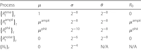
For each single wave, a set of parameters controlling the governing processes is randomly generated using the
parameters in Table 3. The means of the processes for
amplitude and phase variation are sampled according to the following law:
log2μampk ∼U(−1, 1) and μphk ∼U(0, 1)
fork = 1, 2, 3, 4, whereU(a,b)denotes the uniform
dis-tribution on the interval [a,b). They remain constant
throughout the wave and determine the overall shape of the wave.
4.3.2 Generated anomalies
Based on the parameters and processes employed by the wave generator, we inject the following four types of anomalies or noise:
Amplitude anomalies The amplitude process Rampkt t
of one of the frequency components (i.e. for a single
k ∈ {1, 2, 3, 4}) is increased by a, where ais ran-domly sampled for each anomaly according to the law log2a∼U(1, 2).
Phase anomalies The phase process Rphkt t of one of the frequency components is changed. The amount of change is randomly sampled for each anomaly from the distributionU(1/4, 3/4)resulting in a ran-dom phase change of at least 90◦and at most 270◦. Pulse anomalies A pulse of random amplitude is added
onto the wave. For each anomaly, the amplitudepof
the pulse is randomly sampled according to the law
log2p ∼ U(2, 4)and the pulse width is a random
integer drawn from the interval [ 25, 26).
Table 3Parameters for processes governing generated waves (k=1, 2, 3, 4)
White noise The white noise process{Nt}tis amplified
by a factor α which is randomly sampled for each
anomaly according to the law log2α∼U(2, 6).
For each wave, a segment of 216 samples is generated.
Then 16 segments, each consisting of 212samples are
gen-erated, the last 211samples of which the anomaly or noise is injected into. For the evaluation, we use 24 generated waves, resulting in a number of 290 anomalies and 94 waves with increased white noise in the test dataset.
4.3.3 Input data and period detection
The generated waves are considered in 24 groups, where
each group consists of a normal wave recorded over 28=
256 periods and further recordings, each injected with a single type of anomaly with a normal start-up time of at least 211 = 2048 time units (i.e. the first entrance time of anomalies following the respective normal wave is to the
right of the time stamp 211 = 2048). In each group, we
take the first 7/8 and the remainder of the normal wave for training and validation, respectively, and subsequently test the trained classifier on the respective anomaly-injected test recordings.
Since the simulated waves contain interference in the time component which results in random period lengths
s, we again make use of the period detector described in
Appendix A using the parameters specified in Table 4.
Note that in contrast to the treatment of ECG data, in each data group, the reference window is selected among the subpatterns extracted from thetraining data.
By construction, the average period length equalss =
28=256 time units.
4.3.4 Hyperparameters
Throughout the entire training, we set the maximum number of classes and allowed per-class margin of error ton∗0:=10 andα:=2−6, respectively.
As presented in Table1, for each of the 24 waves, the
corresponding classifier neural nets are all endowed with
M(0) = 1 channel and M(1) = 6 channels on the first
and second convolutional layers, respectively, where max
pooling of size R(1) = 3 is applied between the
con-volutional layers, and two fully connected layers are set between the last convolutional layer and the output layer. During the classifier selection process, the lengthT(0) of the input sequence, the sizesS(0),S(2) of the convolution
Table 4Parameters for period detector on wave dataset
Parameter Value
Prefilter window half-lengthn 8
Minimum base period lengthsmin 240
Maximum base period lengthsmax 272
Maximum period length deviation factorσ 1/4
kernels, and the sizeN(3)of the first fully connected layer
vary proportionally to the sliding window length T =
3s/n0 = 768/n0where n0 runs over the values in
{10(= n∗0), 8, 6, 4}if not stopped earlier. The sizeN(4) of the second fully connected layer is the geometric mean of the sizesN(3)andN(5) of its adjacent layers and the size
N(5) of the output layer is equal to the current number
of classesnwhich runs over the values in{n0,n0−1,. . .} during the dynamic reclustering.
The ADAM optimiser with learning rate γ = 0.01 is
employed for training with SGD. The mini-batch sizes are dynamically increased after every 2 or 3 epochs from 40 to 360.
5 Experimental results
In this section, we present the empirical results of the
treatment of the example datasets given in Section4
fol-lowing our general phase classification scheme described in Section3. Here, we provide both the results of selecting and training the optimal classifier neural networks and the results of anomaly detection obtained by evaluating the trained classifier neural networks on the test data (recall Section3.4).
5.1 Cardiology dataset
The ultimate classifier resulting from the dynamic model selection process turns out to be a classifier neural
net-work corresponding to initial number of classesn0 = 6
and final number of classesnn0 = 4, cf. Table5 for the
layout of the final CNN. The label history recorded along
with the dynamic reclustering is shown in Table 6. The
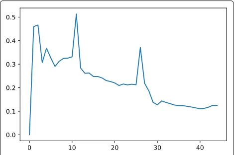
average validation loss recorded during the training of the respective neural nets is presented in Fig.2. A train-ing accuracy of 99% and a validation accuracy of 96% are achieved.
Figures 3 and 4 illustrate the result of testing the
trained classifier on three patients from the category ‘healthy control’ and three ill patients: the measurements on feature ‘i’ from the test patients are presented in a
Table 5Layers of final classifier neural network for ECG dataset
Layer type Sizes
0 Convolutional M(0)=15,T(0)=17,
S(0)=7
1 Max pooling M(1)=90,T(1)=17,
R(1)=3
2 Convolutional M(2)=90,T(2)=6,
S(2)=5
M(3)=270,T(3)=6
3 Fully connected N(3)=1620
4 Fully connected N(4)=80
5 Output N(5)=4
Table 6Label history
Epochs Merge New Labels
0 – 9 N/A [ 0, 1, 2, 3, 4, 5]
9→10 3 to 2 [ 0, 1, 2, 2, 4, 3]
24→25 4 to 2 [ 0, 1, 2, 2, 2, 3]
25 – 43 N/A [ 0, 1, 2, 2, 2, 3]
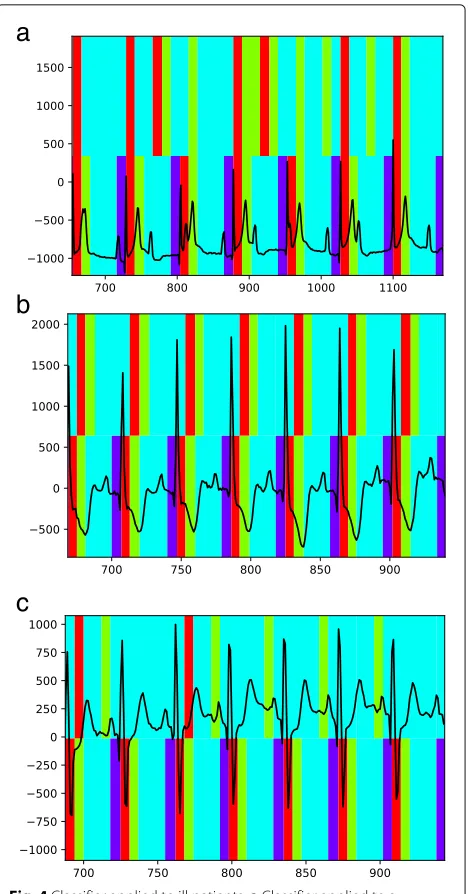
temporal resolution of 20 ms and the bars in the upper and lower halves of the figures refer to the predicted classes and the true labels of the segments from the considered test signals, respectively4.
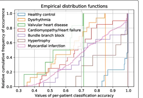
Figure 5 presents a statistical evaluation of the
per-patient test results on per-patients from the seven most recorded categories in the considered database: ‘dys-rhythmia’, ‘valvular heart disease’, ‘cardiomyopathy/heart failure’, ‘bundle branch block’, ‘hypertrophy’, ‘myocardial infarction’, and ‘healthy control’. The lines in different colours represent the empirical distribution functions of the per-patient classification accuracy from the aforemen-tioned categories. Observe that the blue line related to healthy patients is located in the bottom right corner of the diagram, to the left of which all other lines corre-sponding to ill patients are centred (cf. the median for each category), which enables us to distinguish ill patients from healthy patients in some cases. For instance, accord-ing to the figure, if we take the average validation accuracy of 96% as the threshold for the per-patient classification accuracy, all test patients from the categories ‘dysrhyth-mia’ and ‘valvular heart disease’, 90% and nearly 85% of the patients from the categories ‘cardiomyopathy/heart failure’ and ‘myocardial infarction’, respectively, and over 70% of the patients from the categories ‘bundle branch block’ and ‘hypertrophy’ will be considered as anoma-lies, whereas up to three false-positive results (25% of ) all tested patients from the category ‘healthy control’ will be assessed as normal. Since the sample sizes provided
a
b
c
Fig. 3Classifier applied to patients from category ‘healthy control’
for the individual categories vary a lot (e.g. there are 148 subjects for myocardial infarction whereas the entire cate-gory healthy control consists of only 52 subjects including training, validation and test data applied in our context), we are not in the position to make a general statement on
the choice of an ideal threshold value. Table 7provides
a statistical evaluation of the per-disease average classi-fication accuracy. It turns out that the category healthy control presents by far the best test result compared to all other categories related to heart disease (anomaly).
Note that our anomaly detection scheme does not incorporate any specific cardiological knowledge. It gives an indication whether a patient may be ill or not, it detects deviations from the known healthy data and does not classify the diseases separately. It also only gives a
a
b
c
Fig. 4Classifier applied to ill patients.aClassifier applied to a dysrthythmia patient,bClassifier applied to a valvular-heart-disease patient,cClassifier applied to a myocardial-infarction patient
statistical indication, which is a result somewhat similar to the one reported in [31] where it was observed that the ECGs of ill patients showed deviations in certain affine dependencies usually present between the 12-lead and 3-lead ECGs of healthy patients.
5.2 SCADA dataset
The final classifier determined by means of the dynamic
model selection scheme usesn0 = 10 andnn0 = 4, cf.
Table 8 for the layout of the final CNN. The respective
Fig. 5Distribution of per-patient classification accuracy evaluated on test patients from different categories
In Fig.7, the number of active port pairs extracted from ‘test data 1’ is plotted against time (in seconds) and the bars in the upper and lower halves represent the classes predicted by our trained neural net and the true labels of the test segments, respectively; segments which result in prediction errors are considered anomalies.
The final results of our anomaly detection algorithm on
the entire test data are summarised in Table 10. In the
first two (cleaner) test datasets with no or only a small amount of manual operations (noise), all cyber attacks in the test data are detected along with a single false-positive detection (corresponding to 1% false detection rate in ‘test data 1’), whereas the classifier tested on the last test dataset including a large amount of noise performs not as good, which is not surprising taking into account that only malicious activities but no manual operations or any other types of interference are labelled as anomalies and our time series analysis does not include the respective context consideration.
Indeed, the SCADA datasets which are applicable in our setting are quite small. Due to the non-compatibility between datasets with small and large amounts of noise (i.e. non-intrusion anomalies appearing in the form of pulses), it is difficult to choose one suitable dataset for
Table 7Results of per-disease classification accuracy
Disease Classification accuracy (%)
Valvular heart disease 56
Dysrhythmia 60
Cardiomyopathy/heart failure 64
Myocardial infarction 73
Bundle branch block 76
Hypertrophy 86
Healthy control 97
Table 8Layers of final classifier neural network for SCADA dataset
Layer type Sizes
0 Convolutional M(0)=4,T(0)=3,
S(0)=3
1 Max pooling M(1)=24,T(1)=3,
R(1)=1
2 Convolutional M(2)=24,T(2)=3,
S(2)=3
M(3)=72,T(3)=3
3 Fully connected N(3)=216
4 Fully connected N(4)=29
5 Output N(5)=4
training and to test the intrusion detector on datasets with incompatible characteristics, e.g. it would be unfeasible to train an anomaly detector on one of the cleaner datasets and then test it against a noisy dataset, or vice versa. For a more extensive treatment of anomaly detection of type B
described in Section 2.2 using a richer dataset and the
corresponding results, cf. Section4.3and Section5.3.
5.3 Wave dataset
Overall, an average classification accuracy of 99% is achieved on both training and validation data.
Figures 8, 9, 10, and 11 present the detection results of our classifiers trained by individual example waves and tested on segments injected with different types of anomalies and white noise, respectively. Again, in each diagram the bars in the upper and lower halves refer to the predicted classes and true labels of the data from the test segments fed into the trained classifier, respectively. Notice that in Fig.11, slightly increased white noise does not lead to any classification errors, which suggests some robustness property of our classifier against noise.
The final results of our anomaly detection algorithm tested on the 24 groups of synthetic waves are shown
in Table 11. The amount of anomalies and white noise
are obtained by counting the number of test waves injected with the respective type of interference, whereas
Table 9Label history
Epochs Merge New Labels
0 – 34 N/A [ 0, 1, 2, 3, 4, 5, 6, 7, 8, 9]