Blind Equalization of a Nonlinear Satellite System
Using MCMC Simulation Methods
Stéphane Sénécal
Groupe Non-Linéaire, Laboratoire des Images et des Signaux CNRS UMR 5083, LIS-ENSIEG, BP 46, 38402 Saint Martin d’Hères Cedex, France
Email: [email protected] Pierre-Olivier Amblard
Groupe Non-Linéaire, Laboratoire des Images et des Signaux CNRS UMR 5083, LIS-ENSIEG, BP 46, 38402 Saint Martin d’Hères Cedex, France
Email: [email protected]
Received 31 July 2001 and in revised form 12 October 2001
This paper proposes the use of Markov Chain Monte-Carlo (MCMC) simulation methods for equalizing a satellite communication system. The main difficulties encountered are the nonlinear distorsions caused by the amplifier stage in the satellite. Several processing methods manage to take into account the nonlinearity of the system but they require the knowledge of a training/learning input sequence for updating the parameters of the equalizer. Blind equalization methods also exist but they require a Volterra modelization of the system. The aim of the paper is also to blindly restore the emitted message. To reach the goal, we adopt a Bayesian point of view. We jointly use the prior knowledge on the emitted symbols, and the information available from the received signal. This is done by considering the posterior distribution of the input sequence and the parameters of the model. Such a distribution is very difficult to study and thus motivates the implementation of MCMC methods. The presentation of the method is cut into two parts. The first part solves the problem for a simplified model; the second part deals with the complete model, and a part of the solution uses the algorithm developed for the simplified model. The algorithms are illustrated and their performance is evaluated using bit error rate versus signal-to-noise ratio curves.
Keywords and phrases:traveling wave tube amplifier, Bayesian inference, Markov chain Monte-Carlo simulation methods, Gibbs sampling, Hastings-Metropolis algorithm.
1. INTRODUCTION
The importance of telecommunication since the last decade leads to use satellites for transmitting the information. The main drawback of this transmission method is the attenu-ation of the signal due to its trip through the atmosphere. Therefore, one of the aims of the satellite is to “re-amplify” the signal before sending it back to Earth. The lack of space and energy available on the satellite leads to use TWT (Traveling Wave Tube) amplifiers for realising this stage of transmission [1]. Unfortunately, these kinds of amplifiers are intrinsically nonlinear and thus imply complex processing methods for realizing the equalization.
Neural networks inspired methods for modeling and equalizing these communication systems have been success-fully implemented [2, 3, 4]. A Volterra identification cou-pled with a Viterbi receiver has also been studied in [5]. However, these methods need a learning (or training) input sequence for setting the parameters of the equalization
al-gorithm. Some of the recently proposed methods perform successfully the equalization of nonlinear communication channels without the help of such a known input sequence. However, some of these blind methods require special as-sumptions on the emitted signals, Gaussian and circular com-plex random noise in [6] for instance.
Many recent blind methods perform the identification [7] or the equalization [8, 9, 10] of nonlinear communication channels under very general assumptions: they just require that the system can be approached by a finite Volterra filter. Such a modelization is possible for the identification of the model considered here but it does not lead to efficient results for the equalization: it seems that the channel is not reversible by a Volterra filter.
Moreover, all these methods do not take fully into account the prior knowledge available on the emitted signal and on the parametric form of the TWT amplifier [1].
s(t) z(t)
Ndown(t)
Nup(t)
Emission filter
Input
multiplexing TWT
Output multiplexing
Multipath fading channel SATELLITE SYSTEM
Figure1: Satellite communication channel.
of the posterior distribution of the transmitted sequence. This distribution is hardly computable due to the nonlin-earity of the model; but Markov chain simulation methods and Monte-Carlo estimation methods enable to build a for-mal blind equalization algorithm for the considered system. Our aim in this paper is thus to present such an algorithm and its performances on simulated data.
The paper is organized as follows: a brief description of the model is given in Section 2. Considering a simpler model leads to a first Monte-Carlo estimation method of the in-put sequence. This is described in Section 3. In Section 4, the complete model is considered, and we show how to restore the emitted symbols using a Gibbs sampler. This algorithm uses the algorithm specifically designed for the simpler model. Section 5 is devoted to simulations and to the study of the performance of the approach. We conclude the paper by dis-cussing some advantages and drawbacks of the algorithm, and some perspectives of the method.
2. MODELING THE SYSTEM
The model used in the paper is a common model in com-munication using a satellite [4]. This model is depicted in Figure 1. The emitted message is a sequence(sk)1≤k≤nofn
symbols generated at a rateT that passes through an emis-sion filter. For simplicity, we assume that the amplitude of the sequence is constant. The symbols are coded using a known constellation with a known number of states. In this paper, we work with a 4-QAM coding scheme. Thus, the emitted se-quence can be writtensk=Aexp(iφk)where the phase
sam-ples(φk)1≤k≤nare independently and identically distributed
(i.i.d.) from the distribution
φk∼ U{π /4,3π /4,5π /4,7π /4}, (1)
where UΩ denotes the uniform distribution on a set Ω. Note already that the method developed here could easily be adapted to PSK modulations. However, some modifications should be done to handle general QAM modulations to take into account that the amplitudeAis explicitly dependent on φk.
The emitted signal is distorted by the trip through the atmosphere; this is modeled by an additive i.i.d. complex, circular Gaussian noise signalNup(t)
0 0.2 0.4 0.6 0.8 1 1.2 1.4 1.6 1.8 2 1.4
1.2 1 0.8 0.6 0.4 0.2 0
Figure 2: Amplitude gain A(r ) for (αa, βa) = (1.96,0.99)
(straight) and(αa, βa)=(2.15,1.15)(dashed).
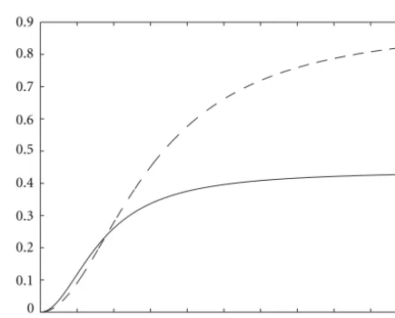
0 0.2 0.4 0.6 0.8 1 1.2 1.4 1.6 1.8 2 0.9
0.8 0.7 0.6 0.5 0.4 0.3 0.2 0.1 0
Figure 3: Phase wrapping Φ(r ) for (αp, βp) = (2.53,2.81)
(straight) and(αp, βp)=(4,9.1)(dashed).
Nup(t)∼ NCC0, σu2
(2)
with varianceσ2
uwhich practically provides a signal-to-noise
ratio (SNR) around 15 dB (the amplitudeAis set at the trans-mitter stage on Earth to reach at least such an SNR).
The signal is then amplified by the satellite and sent back to Earth. This stage is mainly performed by a traveling-wave tube amplifier (TWTA) which can be modeled by the follow-ing amplitude gain and phase wrappfollow-ing [1]:
A(r )= αar
1+βar2, (3)
Φ(r )= αpr
2
1+βpr2, (4)
wherer denotes the input signal amplitude andαa,βa,αp,
andβpare the coefficients of the TWTA model. The functions
Nup(t) Ndown(t)
s(t) x(t) y(t) z(t)
TWTA
Figure4: Simplified communication system.
of the amplitude gain (located over the dotted line in Figure 2) will be considered. It means that for a given output amplitude, the corresponding input amplitude is the smallest one, from which the input phase is also deduced from (4).
Note that the TWT amplifier lies between two IIR linear filters performing the task of multiplexing. The emission filter and the multiplexing filters are modeled by 4-pole Chebychev filters.
The transmission of the signal back to Earth is much less powerful than the previous one because of straight tech-nical constraints of the satellite. Thus, the influence of the atmospheric propagation medium is usually modeled by a linear multipath fading channel [11]. Finally, the signal is additively corrupted by a complex, circular white Gaussian noiseNdown(t)
Ndown(t)∼ NCC
0, σd2. (5)
The signal received is denoted asz(t), and the goal is to re-cover the emitted symbol sequence based on the only knowl-edge of signal z(t)and the type of constellation. Since the problem is difficult, we begin by studying the simpler model depicted in Figure 4. In this model, we focus on the nonlin-earity, and we thus omit the linear filters and the multipath fading channel (downlink transmission). The only perturba-tions considered are the uplink and downlink noises, and of course the effect of the TWTA. The equalization of this simple model is the aim of the following section.
3. RECOVERING THE SYMBOLS: A MONTE-CARLO ESTIMATION METHOD
Given a sequence of samples(z(jTs))1≤j≤m of the received
signal, whereTsstands for the sampling period at the receiver stage, the aim is to estimate the emitted symbol sequence (φk)1≤k≤n. This problem is not trivial even for known
pa-rameters of the TWT amplifier. The effect of the nonlinear TWTA on a constellation of a 4-QAM distributed symbol sequence corrupted by additive noise (SNR =10dB) is de-picted in Figure 5. It appears that the TWTA tends to render the “squared” 4-QAM distributions more circular. A kind of rotating phase effect is also noticeable implying thus a com-plex processing for taking into account its influence.
The first estimation to address is the recovering of the symbol durationT. This can be achieved by usual processing methods such as the study of the autocorrelation function of the received signal z(t)for instance, assuming that the sampling periodTsis short enough and a relatively low
inter-symbol interference.
+
Figure 5: Constellation of the above sequence passed through a TWT amplifier withαa=2,βa=1,αp=4, andβp=9.1.
Figure 6: Autocorrelation coefficients of the received sequence
(z(jTs))1≤j≤mplotted versus delay lags inTsunits (dashed curve for
the real part of the sequence, dash-dotted one for its imaginary part) for uplink SNR=10dB, downlink SNR=5dB,αa=2,βa=1,
αp=4andβp=9.1. The number of samples per symbolp=10
can be estimated as the first zero of the function.
For instance, the autocorrelation function of a received sequence(z(jTs))1≤j≤mis depicted in Figure 6 for an uplink
SNR equal to 10 dB and a downlink SNR equal to 5 dB. This enables us to recover the correct number of observation sam-ples per symbol denoted asp. Given the symbol periodT, or the number p =T /Ts, and assuming a perfect sampling at the receiver system (i.e., thatpis an integer), a first estimation can be performed by a Bayesian approach using the posterior distribution of(φk)1≤k≤n. From Bayes formula and the
The prior distributionp(φk)is known and given by (1); the
main problem is in the calculation of the likelihood
pz(jTs)/φk, A, σu, σd. (8)
By marginalizing with respect toy(jTs)(denoted asyfrom now on, for simplifying notations), expression (8) can be written
y∈Cp
z(jTs), y|φk, A, σu, σddy
∝
y∈Cp
z(jTs)|y, φk, A, σu, σd
×py|φk, A, σu, σddy,
(9)
where we have used Bayes formula. From (5), the first prob-ability density function in the integral in (9) reduces to
pz(jTs)|y, σd
= π σ1 d
exp
−|z(jTs)−y|2
σd2
. (10)
The second density in the integral in (9) is obtained by marginalizing with respect to x(jTs) (denoted as x); this yields
p(y|φk, A, σu, σd)
=
x∈Cp(y, x|φk, A, σu, σd)dx
∝
x∈Cp(y|x, φk, A, σu, σd)
×p(x|φk, A, σu, σd)dx.
(11)
Asy is entirely determined by x from the formal identity y =TWT(x)(see (3) and (4)), the first distribution in the integral in (11) is given by
p(y|x, φk, A, σu, σd)=p(y|x)=δ(y−TWT(x)), (12)
whereδ(·)stands for the usual Dirac distribution. From (2), the second distribution in (11) reduces to
p(x|φk, A, σu)=
1 π σu
exp
−|x−Aexp(iφk)|2
σu2
. (13)
Finally, the likelihood (8) is proportional to
x∈Cp
z(jTs)|TWT(x), σdp(x|φk, A, σu)dx. (14)
This integral cannot be evaluated analytically. Therefore, in order to proceed, we must use some numerical approxima-tions. This leads to the use of Monte-Carlo methods for per-forming a numerical estimation. The expression (14) can be viewed as
E
exp
− 1
σd2|z(jTs)−TWT(x)|
2
, (15)
0 10 20 30 40 50 60 70 80 90 100
0
−2
−4
−6
−8
−10
−12
−14
−16
Figure 7: Computation of thelog of (17) versus the number of samplesN.
where
x∼ NCC
Aexp(iφk), σu2
. (16)
Thus, considering a sequence (x)1≤≤N i.i.d. drawn from
distribution (16), the computation of
1 N
N
=1
exp
− 1
σd2|z(jTs)−TWT(x)|
2
(17)
gives a good approximation of (15) for sufficiently largeN [12]. In practice, few dozens of samplesxienable us to get a
good estimation of (15) and thus of (8). Figure 7 depicts the quantities (17) for a fixed observation samplez(jTs)and for all possible emitted symbolsφk∈ {π /4,3π /4,5π /4,7π /4}
(withk(p−1)+1≤j≤kp). The parameters of the model were set toA=0.5,αa=2,βa=1,αp=4, andβp =9.1
and the signal-to-noise ratios to SNRup=10dB (σu=0.11)
and SNRdown=5dB (σd=0.32). It clearly appears that only
one of the four possible emitted symbols gives a significantly higher numerical estimation of the likelihood. The posterior distribution forφkcan thus be approximated by
φk p(φk|z(jTs), p, A, σu, σd) π
4 3×10⁻¹⁰
3π
4 4×10⁻⁷
5π
4 0.99
7π
4 1×10−
5
The estimated emitted symbol is thus chosen as the one imazing the estimated posterior distribution. Thus, a max-imum a posteriori estimation method can be implemented for realizing the equalization in the case of known TWTA parameters.
We have performed simulations of this method in order to quantify its performances. Figure 8 shows the bit-error-rate (BER) between the emitted symbol sequence(φk)1≤k≤n
and its estimated(φ˜k)1≤k≤ncomputed from the method
sam-0 1 2 3 4 5 6 7
100
10−1
10−2
10−3
10−4
Figure8: BER versus downlink SNR (in dB) computed with the Monte-Carlo estimation method of the posterior distribution pro-posed in Section 3, forp=4(straight) andp=2(dashed).
ples per symbol. Given these parameters, the BER of the pro-posed estimation method appears not to be strongly depen-dent on the input amplitudeAand on the TWTA parameters. Thus, the simulations are run for sequences of a fixed ampli-tudeA=0.3processed by a TWT amplifier whose parame-ters are set toαa=2,βa=1,αp=4, andβp=9.1and the
Monte-Carlo estimations are computed from sequences (16) of 200 samples. The uplink noise variance is also fixed such as SNRup=10dB because in practical communication con-texts, the emitting station on Earth manages to reach such an SNR. The BER curves are computed by averaging the results upon 50 realizations of the algorithm, run for the estimation of sequences of 1,000 4-QAM symbols.
It appears that the BER strongly decreases as the parame-terpincreases, for a fixed downlink SNR. The computation of the probability density function of the posterior distribution is highly dependent on the number of samples at disposal for computing the product (7). Sampling at a rate of one sample per symbol would drastically increase the BER as it would render the estimation of (6) more sensitive to corrupt-ing noise signals. On the contrary, a large number of samples per symbol enables us to reduce considerably this influence and thus to get a robust estimation of (6).
The study of the performances of this Monte-Carlo sim-ulation method has shown its ability to give good estimations of the emitted symbol sequence in the case of a simple TWTA model. This motivates the choice of the Bayesian approach and the estimation of the posterior distribution for process-ing the equalization of the system in the case of unknown TWTA parameters and noise levels.
4. EQUALIZATION WITH MCMC SIMULATION METHODS
4.1. Introduction
If the parameters of the TWTA model described in Section 2 are unknown, the equalization of the communication system described in Figure 1 is quite a nontrivial task. Several
ap-proaches, taking into account the nonlinearity of the system, already exist (cf. Section 1).
The method described hereinafter is devoted to the blind equalization of the channel described in Section 2 by using all the prior knowledge available on the emitted signal and on the parametric form of the nonlinearity. The aim is to estimate jointly the emitted symbol sequence and the parameters of the model. This estimation comes from the posterior distri-bution of interest as exposed previously for the simple system considered in Section 3. For unknown TWTA parameters, the following posterior distribution is considered:
p(φk)1≤k≤n, A, σu, αa, βa, αp, βp, σd|(z(jTs))1≤j≤m
(18) which is very difficult to compute or simulate. A way for studying it is to use Markov chain simulation methods [12, 13]. Their main principle is to draw iteratively a sequence of samples
(φk)1≤k≤n, A, σu, αa, βa, αp, βp, σd
1≤≤N (19)
such that there exists an asymptotic invariant distribution which is precisely the desired posterior distribution (18).
4.2. General algorithm
From the previous success of the Monte-Carlo estimation method for the symbols described in Section 3 and due to the discrete nature of the variables(φk)1≤k≤nand the
multi-dimensionality of the variable to simulate, the Gibbs sampling algorithm [12, 13] is chosen for the implementation and leads to the simulation given in Scheme 1. The simulation steps are described hereinafter.
4.3. Practical implementation
4.3.1 TWTA parameters, noise levels, and amplitude of the emitted signal
From Bayes formula, the posterior distribution (18) is pro-portional to the product of the likelihood
p(z(jTs))1≤j≤m|(φk)1≤k≤n, A, σu, αa, βa, αp, βp, σd
(20) and the prior distribution
p(φk)1≤k≤n, A, σu, αa, βa, αp, βp, σd. (21)
Therefore, the simulation steps of the Gibbs sampling algo-rithm will require the setting of proper prior distributions for the variables (A, σu, αa, βa, αp, βp, σd). Unfortunately,
the likelihood (20) depends on these variables in an implicit way thus rendering impossible the direct simulation of the distributions (S1)–(S7) with a “simple” approach.
• initialize ((φk)k, A, σu, αa, βa, αp, βp, σd)1 according to prior distributions • update ←+1 by drawing
A+1∼pA|((φk)1≤k≤n, σu, αa, βa, αp, βp, σd), (z(jTs))1≤j≤m
(S1)
σu+1∼p
σu|A+1, ((φk)1≤k≤n, αa, βa, αp, βp, σd), (z(jTs))1≤j≤m
(S2)
α+1
a ∼p
αa|(A, σu)+1, ((φk)1≤k≤n, βa, αp, βp, σd), (z(jTs))1≤j≤m
(S3)
β+1
a ∼p
βa|(A, σu, αa)+1, ((φk)1≤k≤n, αp, βp, σd), (z(jTs))1≤j≤m (S4)
α+1
p ∼p
αp|(A, σu, αa, βa)+1, ((φk)1≤k≤n, βp, σd), (z(jTs))1≤j≤m
(S5)
βp+1∼p
βp|(A, σu, αa, βa, αp)+1, ((φk)1≤k≤n, σd), (z(jTs))1≤j≤m
(S6)
σd+1∼pσd|(A, σu, αa, βa, αp, βp)+1, ((φk)1≤k≤n), (z(jTs))1≤j≤m
(S7)
(φk)1≤k≤n
+1
∼p(φk)1≤k≤n|(A, σu, αa, βa, αp, βp, σd)+1, (z(jTs))1≤j≤m
(S8)
Scheme1
a random variable denoted asθ which is distributed from p(θ|(z(jTs))1≤j≤m)for instance.
At iteration+1, a candidateθcis chosen forθ+1, drawn
from a candidate distributionpc(·|θ). This distribution is
usually one of the following two types:
θc∼ Nθ, σc2
, (22)
θc∼ U[θmin,θmax]. (23)
The distribution (22) enables to scan the variable space “little by little.” One of the drawback of this type of candidate dis-tribution is that it is more sensitive to the “stuck” phenomena arising at the localmaximaareas of the probability density function. On the contrary, the type of distribution (23) en-ables to scan theoretically the variable space in its globality even if practically only the candidates drawn in the neigh-borhood of the localmaximaareas of the probability density function are accepted. However, these two types of candidate distribution have the advantage of reducing the complexity of the computation of the acceptance rate (see hereinafter).
Then, given a candidate, an acceptation/rejection process-ing is implemented in Scheme 2.
• generate u∼ U[0,1]
• if u≤α, then set θ+1=θ
c otherwise set θ+1=θ
Scheme2
The acceptance rate is defined byα=min{1, AC}where
AC= p(θc|(z(jTs))1≤j≤m)pc(θ
|θ c)
pc(θc|θ)p(θ|(z(jTs))1≤j≤m)
= m
j=1
p(z(jTs)|θc)pp(θc)
p(z(jTs)|θ)pp(θ)×
pc(θ|θc)
pc(θc|θ)
.
(24)
If a candidate distribution of type (22) has been chosen, a
symmetrical relationpc(θ|θc)=pc(θc|θ)holds. If a
can-didate distribution of type (23) has been chosen, the following holds:
pcθ|θc=pcθ=pc(θc)=pcθc|θ. (25)
Thus theratioabove can be simplified. The distributionpp(·)
denotes the prior distribution of the variableθ. Without any other assumptions on parameterθ, this prior distribution will be assumed to be of the form (23) and thus simplifies also the expression ofAC. Finally, the acceptance rate reduces to the formula
AC= m
j=1
p(z(jTs)|θc)
p(z(jTs)|θ)
(26)
and thus can be computed by Monte-Carlo estimations of likelihood quantities (8) described in Section 3. The same simulation schemes hold for the simulation steps (S1)–(S7).
Practically, upper and lower estimations of the parameter θ are roughly computed at the beginning of the algorithm, leading to the consideration of prior and candidate distribu-tions of type (23). For instance, the variableσuis supposed to
be valued in an interval such that the uplink SNR lies between 10 dB and 15 dB,σdis also supposed to be valued in an
inter-val such that the downlink SNR lies between 0 dB and 10 dB and the prior distribution for the amplitude of the emitted symbols is given by
A∼ U[0.1,0.9]. (27)
The uniform priors for(αa, βa, αp, βp)are settled according
to [1, Table I].
4.3.2 Emitted symbol sequence
As in Section 3, the simulation step (S8) for the symbol se-quence ((φk)1≤k≤n)+1 is performed by a similar
0 0.1 0.2 0.3 0.4 0.5 1.2
1.0 0.8 0.6 0.4 0.2 0
Figure9: Frequency gain of the emission filter (straight), estimation of the power spectrum of the 4-QAM symbol sequence (dashed) and of its associated filtered sequence (dash-dotted) forp=10.
pφk|((φt)1≤t<k, A, σu, ω, σd)+1,
((φt)k<t≤n), (z(jTs))1≤j≤m
(28)
∝ m
j=1
pz(jTs)|((φt)1≤t<k, A, σu, ω, σd)+1,
φk, ((φt)k<t≤n)
×p(φk)
(29)
as the emission and multiplexing stages have to be taken into account for a more realistic modeling. These processing stages are modeled by linear IIR filters (see Sections 2 and 5 for fur-ther details) and fur-therefore imply the appearance of memory in the channel. The simulation step (S8) is thus modified from the method exposed in Section 3 in order to estimate the full posterior distribution of the symbolφkconditionally to the
whole sequence of the observation samples(z(jTs))1≤j≤m.
However, taking fully into consideration that the memory of the system in this simulation step is not compulsory as the filters do not dramatically affect the posterior distribution with strong inter-symbol interference.
For instance, the frequency gain of the emission filter (which has the lowest cut-off frequency of the three IIR fil-ters, see Section 5) is represented in Figure 9 with power spec-trum estimations of a 4-QAM sequence and of its associated filtered sequence. It shows that the emitted signal has mostly a narrow band in the frequency domain and that the emission filter does not affect drastically the symbol sequence as we can observe in the time domain in Figure 10, where samples of the real part of this 4-QAM sequence and of its associated fil-tered sequence are represented. Therefore, the computation of (28) does not seem to require all the observation samples for estimating the value of the probability density function of the posterior distribution for the emitted symbols. Thus, Monte-Carlo estimations of (A.1) have been computed by considering the linear filters for a 4-QAM emission sequence of 100 symbols with 10 samples per symbol and parameters of the system set toA=0.5, SNRup=10dB, SNRdown=5dB with the same TWTA parameters as for the numerical experi-ments in Section 3. These quantities are studied as a function
0 20 40 60 80 100 120 140 160 180 200 0.5
0.4 0.3 0.2 0.1 0
−0.1
−0.2
−0.3
−0.4
−0.5
Figure 10: Some samples of the real part of the 4-QAM symbol sequence (dashed) and of its associated filtered sequence (straight).
400 420 440 460 480 500 520 540 560 580 600 0.6
0.5 0.4 0.3 0.2 0.1 0
Figure 11: Monte-Carlo estimations of (A.1) versus observation samples with φ50 = π /4, considering known symbols φk≠50 (straight) and random symbolsφk≠50(dashed).
of a single symbol and are represented in Figures 11 and 12 for the 50th symbol and various observation samplesz(jTs). It appears firstly that the posterior distribution as a func-tion ofφ50does not depend on the other symbolsφk≠50: the
straight and dashed curves are oscillating around 0.25 for two values ofφ50and for almost all the observation samples. The
variance of these oscillations is of course smaller for exact symbolsφk≠50but in both cases, only the observation
sam-ples roughly located between the 490th and the 510th samsam-ples appear to be relevant for computing the posterior distribu-tion ofφ50. In the simple instantaneous model described in
Section 3, the 491th to the 500th samples had been consid-ered, the delay of the relevant samples attended here comes from the lag indebted by the linear filters.
As a conclusion, the estimation of the posterior distribu-tion of the symbol sequence will be implemented by consid-ering only the samples
z(jTs)
• For k=1 to n do
– For r∈ {1,3,5,7} do
∗ compute numerical approximations of
pz(jTs)|((φt)1≤t<k, A, σu, ω, σd)+1, φk=
π r
4 , ((φt)k<t≤n)
for j=(k−1)p+1+q to kp+q with the Monte-Carlo approximation (17) ∗ estimate (28) for φk=r π4 with the formula
pr= kp+q
j=(k−1)p+1+q
pz(jTs)|((φt)1≤t<k, A, σu, ω, σd)+1, φk=
π r
4 , ((φt)k<t≤n)
and the previous numerical estimations
– compute the values of the cumulative probability density function of the distribution (28)
ˆ
pr=
s≤r ,s∈{1,3,5,7}ps
s∈{1,3,5,7}ps
– end do for r
• draw u∼ U[0,1]
• find r0 as the smallest integer in {1,3,5,7} such as u≤pˆr0 • set φ+1
k = π r0
4
• end do for k
Scheme3
400 420 440 460 480 500 520 540 560 580 600 1.0
0.9 0.8 0.7 0.6 0.5 0.4 0.3 0.2 0.1 0
Figure 12: Monte-Carlo estimations of (A.1) versus observation samples with φ50 = 5π /4, considering known symbols φk≠50 (straight) and random symbolsφk≠50(dashed).
for the kth symbol with a given delay lagq. The setting of this lag will be explained in more details in Section 5. The simulation of step (S8) thus follows Scheme 3.
5. NUMERICAL EXPERIMENTS
The communication model considered for the numerical ex-periments is described in Section 2 and depicted in Figure 1. It is completed from the simple model used in Section 3 de-scribed in Figure 4 by adding emission and multiplexing IIR filters. These ones are modeled by 4-pole Chebychev filters with specific 3 dB bandwidths:1.66/T,2/T, and3.3/T,
re-spectively (see [3, 4, 14]). The downlink transmission model is also completed by a multipath fading channel (cf. [4, 11]) considering one reflected path of 10 dB attenuation.
The equalization method presented in Section 4 was run on simulated data. 50 realizations of 1,000 4-QAM symbols were processed for each given downlink SNR. The parameters of the system were set toA=0.5, SNRup=10dB,αa=2,
βa=1,αp =4, andβp=9.1. For each realization, 100
it-erations of the Gibbs sampling algorithm were run and the estimations from the posterior distribution were taken from the last 50 iterations. Of course, the convergence of the global Markov chain for all the variables to simulate may not be completely reached after 50 iterations of the Gibbs sampling algorithm but the simulation of the symbol sequence gives always the same results after the first dozen iterations. This is mainly due to the robustness of the Monte-Carlo estimation method for the posterior distribution of the symbol sequence described in Section 3. It appeared that these estimated poste-rior probabilities do not depend too strongly on the emitted signal amplitude and the TWTA parameters. This point is discussed in the appendix.
0 1 2 3 4 5 6
10−1
10−2
10−3
10−4
10−5
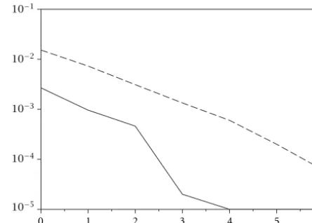
Figure13: BER versus downlink SNR (in dB) for the MCMC equal-ization method forp=8andq=2(straight),q=3(dashed),q=4
(short dash-dotted), andq=5(long dash-dotted).
0 0.4 0.8 1.2 1.6 2.0 2.4 2.8 3.2
10−1
10−2
10−3
10−4
10−5
Figure14: BER versus downlink SNR (in dB) for the MCMC equal-ization method forp=12andq=3(straight),q=4(dashed),
q=5(short dash-dotted), andq=6(long dash-dotted).
The performances of the MCMC equalization method are studied in terms of bit error rates for various downlink SNR. A first task to address is the setting of the delay lagqin the simulation step (S8). Given a sampling rate ofp=8samples per symbol period, the BER curves for various delay lagsq are depicted in Figure 13. It appears that the lag performing the best error rates for this particular number of samples per symbol isq=3. BER performances forq=4are also similar to the ones forq = 3, but the performances are corrupted if a lag greater thanq=4is chosen. If we consider a larger number of samples per symbol, for instancep=12, the delay lag minimizing the BER isq=6(cf. Figures 14 and 15).
Experimenting various even numbers of samples per symbolp, we have observed thatq =p/2usually gives the best BER performances. Thus, the memory of the channel induced by the linear filters is compensated in the process-ing method by a proper delay lag of the observation samples q=p/2for known symbol period.
0 1 2 3 4 5 6
10−1
10−2
10−3
10−4
10−5
Figure15: BER versus downlink SNR (in dB) for the MCMC equal-ization method forp=12andq=6(straight),q=7(dashed), andq=8(dash-dotted).
0 1 2 3 4 5 6
10−1
10−2
10−3
10−4
10−5
Figure16: BER versus downlink SNR (in dB) for the MCMC equal-ization method forp =12andq =6(straight), andp=8, and
q=4(dashed).
For this delay lag, we have run 100 simulations of 500 Gibbs sampling iterations each on 1,000 symbols se-quences. The BER performances (averaged from the 400th to the 500th Gibbs iterations and upon the realizations) for p = 8andp =12are depicted in Figure 16. It shows that a large number of samples per symbol period enables to increase the BER performances as it was the case for the estimation Monte-Carlo method described in Section 3 (cf. Figure 8).
Unfortunately, for this blind equalization method, pro-cessing a large amount of samples increases drastically the computing time as for each iteration of the Gibbs sam-pling algorithm, the computation of an acceptance rate of a Hastings-Metropolis algorithm requires the estimation of likelihood quantities (8) by Monte-Carlo simulation methods many times, in the order of twice the size of the observation sequence.
βa, αp, βp, σd)requires a large number of Gibbs sampling
iterations in practice due to the robustness of the Monte-Carlo estimation method of the likelihood quantities (8).
Therefore, if we are not interested by the “identification” aspect of the processing method but more by the recovering of the symbol sequence, a formal blind estimation method can be built from the Monte-Carlo simulation method in Section 3. A natural way for processing the blind case with-out estimating the parameters is to use the posterior distribu-tion of the emitted symbols by integrating out the parameters (A, σu, αa, βa, αp, βp, σd), considered here as nuisance
pa-rameters. This approach is developed in the appendix.
6. CONCLUSION AND PERSPECTIVES
The blind equalization method presented here showed signif-icant success when it was applied to a common TWTA satellite communication system. Provided good synchronization and estimation of the symbol rate, the MCMC simulation method manages to reach appreciable bit error rates when appropriate delay-lag have been settled for the estimation of the emitted symbol sequence. This lag depends directly on the number of samples per symbol and thus on the estimation of the symbol period.
One of the drawbacks encountered is of course the high demand in time-computing for the processing, especially for the simulation steps of the Gibbs sampling algorithm con-cerning the amplitude of the emitted signal, the noise levels and the TWTA parameters. Indeed, for each of these steps and at every iteration of the Gibbs sampler, the number of Monte-Carlo simulations of (15) is of the order of the length of the observation sequence.
Another drawback, but which can also be viewed as an advantage, is the robustness of the Monte-Carlo estimation method of the likelihood (8) for variable parameters (ampli-tude of the emitted signal, the noise levels, and the TWTA parameters). This tends to slow the mixing property of the Gibbs sampling algorithm. It is then difficult to get precise estimations of the amplitude of the emitted signal, the noise levels and the TWTA parameters with the MCMC equaliza-tion described previously but the uniform prior distribuequaliza-tions set for these parameters are sufficient for running the Gibbs sampling algorithm for a few dozens iterations and for reach-ing an appreciable BER with the estimated symbol sequence from the posterior distribution.
The algorithm will have to be run on real data for com-paring its performances to other equalization methods. The method proposed in this paper could also be extended for solving the equalization problem without knowing the sym-bol periodT by including the parameterpas a component of the variable of the posterior distribution (18). Then, the MCMC implementation would require the use of model se-lection simulation methods (cf. [15] for a review) for drawing samples from a random variable whose dimension also has to be estimated. These kinds of general approaches could also be applied to the estimation of the modulation type and of the transmission system from sets of different classes of para-metric models.
0 100 200 300 400 500 600 700 800 900 1000 0.13
0.11 0.09 0.07 0.05 0.03 0.01
FigureA.1 Computation of (17) versus the number of samplesN.
APPENDIX
BUILDING A MONTE-CARLO SIMULATION METHOD FOR THE BLIND CASE
We consider the simplified model depicted in Figure 4 and try to estimate the emitted symbol sequence con-sidering that the parameters of the transmission channel (A, σu, αa, βa, αp, βp, σd)are unknown.
Although the estimation method proposed in Section 3 is robust for these parameters (for some parameters fixed in a neighborhood of the real values, the estimation (17) remains efficient), it could be very inefficient for some arbitrary fixed values. For instance, if we consider the same computation of the likelihood quantities for a fixed observation sample as in Section 3 (Figure 7) but using the parameters set toA=0.1, αa = βa = αp = βp = 1, andσu = σd = 0.5, then the
Monte-Carlo estimation method would lead to inexploitable results. The estimation of the expectation (15) is depicted in Figure A.1 and the posterior distribution of φk can be
approximated by
φk p(φk|z(jTs), p, A, σu, σd) π
4 0.19
3π
4 0.28
5π
4 0.29
7π
4 0.23
A natural approach would be then to consider a maximum a posteriori estimation from the distribution
p(φk|(z(jTs))1≤j≤m, p) (A.1)
which can be computed by marginalizing with respect to the unknown parameters
pφk, A, σu, αa, βa, αp, βp, σd|(z(jTs))1≤j≤m, p
=
pφk|(z(jTs))1≤j≤m, p, A, σu, αa, βa, αp, βp, σd
×pA, σu, αa, βa, αp, βp, σd)d(A, σu, αa, βa, αp, βp, σd.
(A.2)
This integral can be approximated with a Monte-Carlo scheme by generating a sequence(A, σu, αa, βa, αp, βp, σd)
from the prior distributionp(A, σu, αa, βa, αp, βp, σd)for
1≤≤Nand computing
1 N
N
=1
pφk|(z(jTs))1≤j≤m,
p, Al, σu,l, αa,, βa,, αp,, βp,, σd,
.
(A.3)
A reasonable hypothesis for the prior distribution is to assume the parameters independent and uniformly distributed from
A∼ U[0,1],
σu∼ U[0,0.5],
αa∼ U[0,2.5],
βa∼ U[0,1.2],
αp∼ U[0,4.1],
βp∼ U[0,9.2],
σd∼ U[0,0.7],
(A.4)
where the support of the distributions are chosen from prac-tical considerations: the amplificative part of Figure 2 forA, bounds computed from maximum admissible values forA and uplink and downlink SNR forσuandσdand maximum
values for(αa, βa, αp, βp)found in the tables in [1] for
de-scribing various kinds of TWT amplifiers.
For each sample(A, σu, αa, βa, αp, βp, σd), the
quan-tity to compute in (A.3) is
pφk|(z(jTs))1≤j≤m, p, A, σu,, αa,, βa,, αp,, βp,, σd,
∝p(z(jTs))1≤j≤m|φk, p, A,
σu,, αa,, βa,, αp,, βp,, σd,
×p(φk)
∝ kp
j=(k−1)p+1
pz(jTs)|φk, p, A,
σu,, αa,, βa,, αp,, βp,, σd,
×p(φk).
(A.5)
From the formulae (8), (15), and (17) developed in Section 3, the likelihood expression in the product (A.5) can be com-puted from the following Monte-Carlo approximation:
1 Nx
Nx
q=1
1 σd,2 exp
− 1
σd,2 |z(jTs)−TWT(xq)|
2
, (A.6)
where (xq)1≤q≤Nx is a sequence drawn i.i.d. from distri-butionNCC(Aexp(iφk), σu,2 ).
The Monte-Carlo estimations of (A.1) are much im-proved by this approach by averaging over all possible values of the parameters than by fixing arbitrary values for them, even for raw estimations of (A.6) by sampling onexfor every
0 100 200 300 400 500 600 700 800 900 1000 0.12
0.10 0.08 0.06 0.04 0.02 0
FigureA.2: Computation of (A.1) versus the number of samplesN
(Nx=1).
sample(A, σu, αa, βa, αp, βp, σd). These averaged
estima-tions for a fixed observation sample as in Section 3 (Figure 7) are depicted in Figure A.2 and the estimation for the posterior distribution ofφkis then given by
φk p(φk|z(jTs)) π
4 0.01
3π
4 0.13
5π
4 0.81
7π
4 0.02
This Monte-Carlo simulation method thus gives a way to per-form the blind equalization of the simple channel depicted in Figure 4. However, in a realistic case, the whole transmis-sion chain (cf. Figure 1) has to be considered and also the convergence of this Monte-Carlo method has to be clearly established.
ACKNOWLEDGEMENTS
The authors wish to thank the reviewers for their helpful com-ments. The first author wishes to thank W. T. Chang, W. R. Wu, and Y. T. Su from the Departement of Communication of National Chiao Tung University, Taiwan, for their welcom-ing and advices and also K. Raoof, M. A. Khalighi, and L. Ros from LIS for their precious comments.
REFERENCES
[1] A. A. M. Saleh, “Frequency-independent and frequency-dependent nonlinear models of TWT amplifiers,”IEEE Trans-actions on Communications, vol. COM-29, no. 11, pp. 1715– 1720, 1981.
[2] G. J. Gibson, S. Liu, and C. F. N. Cowan, “Multilayer perceptron structure applied to adaptative equalisers for data communica-tion equalizers,” inProceedings IEEE of ICASSP, pp. 1183–1186, 1989.
IEEE transactions on signal processing, vol. 46, no. 5, pp. 1208– 1220, 1998.
[4] S. Bouchired, M. Ibnkahla, D. Roviras, and F. Castanié, “Equal-ization of satellite mobile communication channels using rbf networks,” inProceedings of Personal Indoor and Mobile Radio Communication, September 1998.
[5] J. Y. Huang, “On the design of nonlinear satellite cdma receiver,” M.S. thesis, Institute of Communication Engineering, College of Engineering and Computer Science, National Chiao Tung University, Taiwan, June 1998.
[6] S. Prakriya and D. Hatzinakos, “Blind identification of LTI-ZMNL-LTI nonlinear channel models,” IEEE Transactions on Signal Processing, vol. 43, no. 12, pp. 3007–3013, 1995. [7] S. Prakriya and D. Hatzinakos, “Blind identification of linear
subsystems of LTI-ZMNL-LTI models with cyclostationary in-puts,”IEEE Transactions on Signal Processing, vol. 45, no. 8, pp. 2023–2036, 1997.
[8] G. Kechriotis, E. Zervas, and E. S. Manolakos, “Using recur-rent neural networks for adaptative communication channel equalization,” inIEEE Transactions on Neural Networks, March 1994.
[9] G. B. Giannakis and E. Serpedin, “Linear multichannel blind equalizers of nonlinear fir Volterra channels,” IEEE Transac-tions on Signal Processing, vol. 45, no. 1, pp. 67–81, 1997. [10] G. M. Raz and B. D. Van Veen, “Blind equalization and
iden-tification of nonlinear and IIR systems—a least squares ap-proach,”IEEE Transactions on Signal Processing, vol. 48, no. 1, pp. 192–200, 2000.
[11] C. Myer, M. Moeneclay, and S. A. Fechtel,Digital Communica-tion Receivers, Wiley series in telecommunications and signal processing. Wiley, 1995.
[12] C. P. Robert and G. Casella, Monte Carlo Statistical Methods, Series in Statistics. Springer-Verlag, 1999.
[13] J. S. Liu, Monte-Carlo Strategies in Scientific Computing, Springer series in Statistics. Springer, 2001.
[14] A. V. Oppenheim and R. W. Schafer,Discrete-Time Signal Pro-cessing, Prentice-Hall signal processing series. Prentice-Hall, 1989.
[15] C. Andrieu, P. M. Djuric, and A. Doucet, “Model selection by mcmc computation,” Signal Processing, vol. 81, no. 1, pp. 19–37, 2001.
Stéphane Sénécal received the M.S. and DEA degrees in 1999 from the Institut National Polytechnique, Grenoble, France, where he is now applying for a Ph.D. de-gree at the Laboratoire des Images et des Sig-naux (LIS CNRS UMR 5083). His research interests include Markov chain Monte Carlo methods and nonlinear modeling and pro-cessing.
Pierre-Olivier Amblardwas born in Dijon, France, in 1967. He received the Ingénieur degree in electrical engineering in 1990 from the ENSIEG-INPG. He received the DEA de-gree and the Ph.D. thesis in signal processing in 1990 and 1994, both from the INPG. Since 1994, he has been Chargé de Recherches with the Centre National de la Recherche Scien-tifique (CNRS), and he is working in the