Available online:
https://pen2print.org/index.php/ijr/
P a g e | 404Burr type III Software Reliability Growth Model with
Interval Domain Data
Dr R.Satya Prasad
1, N.Krishna Kumar
2, Dr G Sridevi
3Professor, Dept. of CSE, Acharya Nagarjuna University.Guntur.
Assoc.Professor, Dept. of MCA, Krishna Chaitanya Institute of Science & Technology,Nellore.
Professor, Dept. of CSE, Malla Reddy Institute of Technology, Hyderabad.
Abstract:
To assess software reliability, there are many software reliability growth models (SRGMs) have been proposed in the past four decades. In principle, two widely used methods for the parameter estimation of SRGMs are the maximum likelihood estimation (MLE) and the least squares estimation (LSE).This paper presents Burr type III software reliability growth model based on Non Homogenous Poisson Process (NHPP) with interval domain data. The ML Estimation method is used for finding unknown parameters in the model. The method of performance analysis of developed software with different data software failure data. How good does a mathematical model fit to the data is also being calculated. To access the performance of the considered SRGM, we have carried out the parameter estimation on the real software failure datasets.
Keywords
Software Reliability, NHPP, Burr type III distribution, Interval domain data, ML Estimation
1.
Introduction
One of the most difficult problems of software industry is to ship a reliable product. Therefore it is necessary to have accurate and fast estimation techniques for verifying software reliability. Software reliability assessment is important to evaluate the quality of software system, since it is one of the most important attribute of software. For Four decades, many Software Reliability Growth Models (SRGMs) have been proposed in estimating reliability growth of software products. SRGMs can be used to depict the behaviour of observed software failures characterized by either
times of failures (i.e Time domain data) or by the number of failures at fixed times (i.e Interval domain data) (Lyu, 1996).
The parameters of SRGMs are generally unknown and have to be estimated based on collected failure data. Two of the most popular estimation techniques are Maximum Likelihood Estimation (MLE) and Least Squares Estimation (LSE) (Goel, 1985; Ohba, 1984). The method of MLE estimation by solving a set of simultaneous equations and is better in deriving confidence intervals. The method of LSE minimizes the sum of squares of the deviations between what we actually observe and what we expect. Nevertheless, LSE is suitable for fitting data from small to medium sample sizes (Wood, 1996), while MLE is considered to be better statistical estimator for large sample sizes. In particular, when the formulated model of SRGMs is complicated or the sample size of failure data is large, these two estimation techniques may not be effective to find out the optimal solutions and generally require to be solved numerically. Hence, the more effective and applicable approaches for the parameter estimation of SRGMs may be necessary. The genesis and the development of the model with the necessary input about a Non Homogenous Poisson Process are presented in Section 2. Proposed model description is presented in Section 3. Illustrating the Maximum likelihood (ML) estimation is given in Section 4. The method of performance analysis is given in Section 5 and Summary and Conclusions are given in Section 6.
2.
NHPP Model
Available online:
https://pen2print.org/index.php/ijr/
P a g e | 405issue in the NHPP model is to determine an
appropriate mean value function to denote the expected number of failures experienced up to a certain time point. There are numerous software reliability growth models available for use according to probabilistic assumptions. Model parameters can be estimated by using maximum Likelihood Estimate (MLE). NHPP model formulation is described in the following lines.
A software system is subjected to failures at random times caused by errors present in the system. Let
N t t
( ),
0
be a counting process representing the cumulative number of failures by time ‘t’, where t is the failure intensity function, which is proportional to the residual fault content.Let
m t
( )
represent the expected number of software failures by time ‘s’. The mean value functionm t
( )
is finite valued, non-decreasing, non-negative and bounded with the boundary conditions.0,
0
( )
,
t
m t
a t
Where ‘a’ is the expected number of software errors to be eventually detected.
Suppose
N t
( )
is known to have a Poisson probability mass function with parametersm t
( )
i.e.,
(
( )!
) .
( )
,
0,1, 2...
n m t
m t
e
P N t
n
n
n
Then
N t
( )
is called an NHPP. Thus the stochastic behaviour of software failure phenomena can be described through theN t
( )
process. Various time domain models have appeared in the literature that describes the stochastic failure process by an NHPP which differ in the mean value functionm t
( )
.Then the stochastic behavior of software failure phenomenon can be described through the N(t) process. In this paper we consider m(t) as given by
( )
1
c bm t
a
t
3.
Proposed Model Description
Burr (1942) had introduced twelve different forms of cumulative distribution functions for modeling data. The task of building a mathematical model is incomplete until the unknown parameters i.e. the model parameters are estimated and validated on actual software failure data sets. In this section we develop expressions to estimate the parameters of the Burr type III model based on Interval domain data. Parameter estimation is given primary importance for software reliability prediction. Parameter estimation can be achieved by applying a technique of MLE which is the most important and widely used estimation technique. A set of failure data is usually collected in one of two common ways, time domain data and interval domain data. Here the failure data is collected through interval domain data
.
The mean value function and intensity function of Burr Type III NHPP model are as follows. The Cumulative distributive function (CDF) is given by
( )
1
c bm t
a
t
Where t>0Let 𝑆𝑘 be the time between (𝑘 − 1)𝑡ℎ and 𝑘𝑡ℎ failure
of the software product. Let 𝑋𝑘 be the time up to the
𝑘𝑡ℎ failure. Let us find out the probability that time
between (𝑘 − 1)𝑡ℎ and 𝑘𝑡ℎ failures, i.e., 𝑆
𝑘 exceeds a
real number ‘s’ given that the total time up to the
(𝑘 − 1)𝑡ℎ failure is equal to 𝑥.
i.e.,
𝑃 [𝑆
𝑘>
𝑠𝑋𝑘−1
= 𝑥]
𝑅 𝑆𝑘/𝑋𝑘−1(𝑠/𝑥) = 𝑒−[𝑚(𝑥+𝑠)−𝑚(𝑠)]
This Expression is called Software Reliability.
4.
Illustrating the ML Estimation
Available online:
https://pen2print.org/index.php/ijr/
P a g e | 406A set of failure data is usually collected in one of
two common ways, time domain data and interval domain data. In this paper parameters are estimated from the interval domain data.
The mean value function of Burr type III model is given by
( )
1
c bm t
a
t
(1)In order to have an assessment of the software reliability, a, b and c are to be known or they are to be estimated from software failure data. Expressions are now delivered for estimating ‘a’, ‘b’ and ‘c’ for the Burr type III model.
Assuming the given data are given for the cumulative number of detected errors ni in a given time interval (0,
ti) where i=1,2, ….. n and 0 < t1< t2< …tn, then the
logarithmic likelihood function (LLF) for interval domain data is given by
1 1
1
(
)log
( )
(
)
( )
k
i i i i k
i
LogL
n
n
m t
m t
m t
(2) Substituting m(t) in the above equation, we get
1 1
1
( ) log 1 1
1
k b b
c c
i i i i
i b c k
LogL n n a t a t
a t
Taking the Partial derivative with respect to ‘a’ and equating to ‘0’.
0
Log L
a
1 1(
) 1
k b
c
i i k
i
a
n
n
t
(3) The parameter ‘b’ is estimated by iterative Newton
Raphson Method using
𝑏𝑛+1= 𝑏𝑛− 𝑔(𝑏)
𝑔′(𝑏) , Where 𝑔(𝑏)𝑎𝑛𝑑 𝑔′(𝑏) are expressed as follows.
𝑔(𝑏) =
𝜕𝐿𝑜𝑔𝐿𝜕𝑏
= 0
1 1 1 11 1 1 1
1 1 1
1 1
1
1
(1
) log(1
) (1
) log(1
)
log 1
log(1
)
(1
)
(1
)
( )
(n
)
1
log
1
b b
i i i i
i i b b
k
i i
i i
i
k
t
t
t
t
t
t
t
t
Log L
g b
n
b
t
(4)Again partial differentiating with respect to ‘b’ and equate to 0 , we get
2 '
2
( )
LogL
0
g b
b
Available online:
https://pen2print.org/index.php/ijr/
P a g e | 4071 1
1 1 1
1 1 1
1 2
1
' 1 1 2
2 1
1
1
1
(1
) (1
) log
log
1
1
(
)
( )
(1
)
(1
)
b b i i
i i i i k i i b b i i i
t
t
t
t
t
t
n
n
LogL
g b
t
t
b
(5)
The parameter ‘c’ is estimated by iterative Newton Raphson Method using
𝑐
𝑛+1= 𝑐
𝑛−
𝑔(𝑐𝑛)𝑔′(𝑐𝑛)
Where 𝑔(𝑐) 𝑎𝑛𝑑 𝑔′(𝑐) are expressed as follows.
( )
LogL
0
g c
c
1 1 1 11 1 1
1
1
1
log
log
1
1
( )
(
)
log
log
1
1
1
1
(n
)
log
1
c c i i c c k i i i ii i c c c c
i i i i i i i
c k
i i c
k k
t
t
t
t
t
t
LogL
g c
n
n
c
t
t
t
t
t
t
t
n
t
t
1 k i
(6) 2 2 2 ' 1 1
2 2 2
1 1 1
2 1 1 1 2 2 1 1 1
1
1
( )
(
) log
log
(1
)
(1
)
1
log
log
(
) log
(
)
(1
)
c c
k
i i
i i c c
i i i i i
c c c
i i i i k
i i
c c c
i
i i i i k k
t
t
Log L
g c
n
n
c
t
t
t
t
t t
t
t
t
n
n
t
t
t
t
t
t
k
(7)5.
Data Analysis
Available online:
https://pen2print.org/index.php/ijr/
P a g e | 408taken from Wood (1996) consists of the observation
time (week), CPU hours and the number of failures detected per week : defects found.
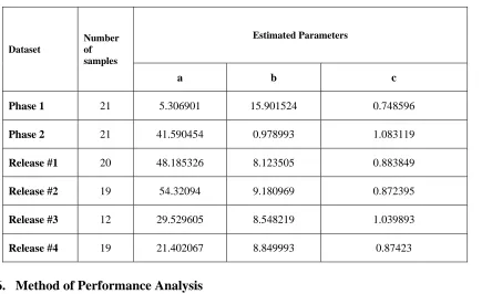
Table 1: Parameters estimated through MLE
Solving equations by Newton Raphson method (N-R) method for all the data sets, the iterative solutions for MLE’s of a,b,c of given software failure datasets are shown in Table 1.
Dataset
Number of samples
Estimated Parameters
a b c
Phase 1 21 5.306901 15.901524 0.748596
Phase 2 21 41.590454 0.978993 1.083119
Release #1 20 48.185326 8.123505 0.883849
Release #2 19 54.32094 9.180969 0.872395
Release #3 12 29.529605 8.548219 1.039893
Release #4 19 21.402067 8.849993 0.87423
6.
Method of Performance Analysis
The performance of SRGM is judged by its ability to fit the software failure data. The term goodness of fit denotes the question of “How good does a mathematical model fit to the data?”. In order to validate the model under study and to assess its performance, experiments on a set of actual software failure data have been performed. The performance evaluation of software reliability growth model is generally measured with sum of square errors (SSE) and correlation index of regression curve equation (R-square). Among them, the model performance is better when SSE is smaller and R-square is close to 1. SSE is used to describe the distance between actual and estimated number of faults detected totally, which is defined as
21
( )
n
i i
i
SSE
y
m t
(8)
Where n denotes the number of failure samples in failure data set,
i
y
denotes the number of faults observed to the momenti
t
, andm t
( )
i denotes theestimated number of faults detected to the time
Available online:
https://pen2print.org/index.php/ijr/
P a g e | 409The equation of calculating the value R-square is
written as:
2
1
2
1
( )
n
i i
n
i i
y m t
R
square
y y
Where
y
denotes the mean value of faults detected.
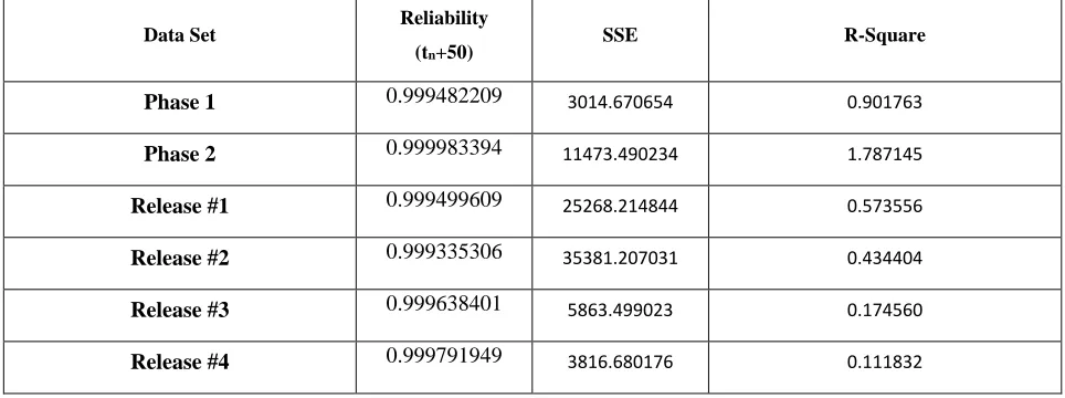
The model can provide a better goodness-of-fit when the value of R-square is close to 1. The reliabilities and performance of the different data sets are presented in Table 2.
Table 2. The results on different data sets
Data Set Reliability
(tn+50)
SSE R-Square
Phase 1 0.999482209 3014.670654 0.901763
Phase 2 0.999983394 11473.490234 1.787145
Release #1 0.999499609 25268.214844 0.573556
Release #2 0.999335306 35381.207031 0.434404
Release #3 0.999638401 5863.499023 0.174560
Release #4 0.999791949 3816.680176 0.111832
From the Table -2 it can be seen that the value of SSE is smaller and the value of R-square is more close to 1. The results indicate that our NHPP Burr type III distribution model based on fault detection rate fits the data in the given datasets, best and predicts the number of residual faults in software most accurately.
7.
Conclusion
In this paper the fault detection rate is calculated with the number of faults remaining in the software. Considering the two factors jointly the fault detection rate is more realistic and accurate. Moreover, we have discussed the performances of 6 datasets by using our new Burr type III SRGM. The experiment result shows that the Phase 1 data set can provide a better goodness-of-fit compared with other datasets. The reliability of
the model over Release #4 data is high among the data sets which were considered.
8.
References
[1] Lyu, M. R. Handbook of Software Reliability Engineering, McGraw-Hill, 1996.
[2] Goel, A. L. (1985). "Software Reliability Models: Assumptions, Limitations, and Applicability," IEEE Transactions on Software Engineering, vol. 11, no. 12, pp. 1411-1423.
[3] Ohba, M. (1984). "Software Reliability Analysis Models," IBM Journal of Research and Development, vol. 28, no. 4, pp. 428- 443.
[4] Wood, A. (1996). "Predicting Software Reliability," IEEE Computer, vol. 29, no. 11, pp. 69-77.
Available online:
https://pen2print.org/index.php/ijr/
P a g e | 410[6] Goel, A.L., Okumoto, K., 1979. Time-dependent error detection rate model for software reliability and other performance measures. IEEE Trans. Reliab. R-28, 206-211.
[7] Pham. H., “System Software Reliability”, Springer 2006.
[8] Burr (1942), “Cumulative Frequency Functions”, Annals of Mathematical Statistics, 13, pp. 215-232.