www.ijiset.com
Bayesian Approach in Estimation of Shape and
Scale Parameter of Log-Weibull model
Dr. Ashwini Kumar Srivastava
Department of Computer Application, Shivharsh Kisan PG College Basti, U.P., INDIA
Abstract
The Log-Weibull model is obtained when the logarithm of a nonnegative random variable follows the Weibull model. This paper examines the possibility and appropriateness for it to be used as a lifetime distribution. In order to get a better understanding of our Bayesian analysis, we consider Markov chain Monte Carlo (MCMC) simulation method to estimate the parameters of Log-Weibull model based on a complete sample under uniform prior. A procedure is developed to achieve our outcome, in OpenBUGS and required all statistical analyses are done by using language R with real data set.
Keywords:
Log-Weibull model31T, 31TBayesian analysis31T, 31TOpenBUGS31T, 31TMCMC) simulation study31T.1. Introduction
Let the random variable X follows Weibull model with parameters α and β then Z =μ + σβ (log X – log α)
follows the Log-Weibull model with location parameter μ and scale parameter σ. Since X ~W(α, β) its probability density function can be written as
1 x
f (x; , ) x . exp ; ( , ) 0, x 0.
β β−
β
β
α β = − α β > >
α
α
Now, the transformation
z = μ + σβ (log x – log α) gives
1 z z
f (z; , )µ σ = exp − µ . exp−exp − µ ; − ∞ < < ∞ σ >z , 0.
σ σ σ
which the probability density function of Log-Weibull model with location parameter μ and scale parameter σ.
Parameter estimation of the Log–Weibull model can be viewed as a special case of the estimation for extreme value distributions. Dekkers et al. [2] and Christopeit [1] have investigated estimation by the method of moments. More information about statistical inference is provided in the monograph by Kotz and Nadarajah [6]. The first, but still noteworthy case study applying the Log–Weibull model as the lifetime distribution for ball bearing was done by Lieblein and Zelen [8]. An excellent review of Log–Weibull model is given by Johnson, Kotz et al.[3, 4.7], Klugman et al.[5], Marshall and Olkin [10] and Rinne[12]. We note that the relationship between Weibull and Log–Weibull variables is the reverse of that between normal and log–normal variables. That is, if log X is normal then X is called a log-normal variable, while if exp(Y) has a Weibull model then we say that Y is a Log–Weibull variable. Perhaps a more appropriate name than Log–Weibull variable could have been chosen, but on the other hand one might also argue that the name “log-normal” is misapplied.
2. Model Analysis
The Probability density function (pdf) of Log-Weibull model with shape parameter μand scale parameter σis
1 x x
f (x; , )µ σ = exp − µ . exp−exp − µ ; − ∞ < < ∞ σ >x , 0.
σ σ σ (1)
The Log-Weibull model will be denoted by LW(μ,σ) [9]. The corresponding Cumulative distribution function
www.ijiset.com x
F(x; , )µ σ = 1 − exp−exp − µ ; − ∞ < < ∞ σ >x , 0.
σ
(2)
The R functions dlog.weibull( ) and plog.weibull( ) develop to be used for the computation of pdf and cdf, respectively. Some of the typical LW density functions for different values of σ and for μ = 5 are depicted in Figure 1 which shows that the density function of the LW(μ,σ) can take different shapes. The Log–Weibull density is negatively skewed with a mode x= μ.
Fig. 1: Plots of the probability density function of the Log-Weibull model
The reliability/survival function is given by x
R(x; , )µ σ = exp−exp − µ ; − ∞ < < ∞ σ >x , 0.
σ
(3)
The R function slog.weibull( ) develop to be used for the computation of the reliability/ survival function[14]. The hazard rate function(hrf) is given by
1 x
h(x; , )µ σ = exp − µ
σ σ (4)
The hazard rate is an increasing function. It has been graphed in Figure 2for shape parameter μ=5 and different values of scale parameter σ by using self developed R function hlog.weibull( ) .
www.ijiset.com The cumulative hazard function H(x) defined as
{
}
H(x)= − −1 log F(x) (5)
can be obtained with the help of self developed R function plog.weibull( ) by choosing arguments lower.tail=FALSE and log.p=TRUE. i.e.
- plog.weibull(x, mu sigma, lower.tail=FALSE,log.p=TRUE)
Two other relevant functions useful in reliability analysis are failure rate average (fra) and conditional survival function (crf). The failure rate average of X is given by
x
0 h(x) dx H(x)
FRA(x) =
x x
∫
= , x > 0, (6)
where H(x) is the cumulative hazard function. An analysis for FRA(x) on x permits to obtain the IFRA and DFRA classes. The survival function and the conditional survival of X are defined by
R(x)= 1 − F(x)
and R (x | t) = R (x + t)
R(x) , t > 0, x > 0, R (·) > 0, (7)
respectively, where F(·) is the cdf of X. Similarly to h(x) and FRA(x), the distribution of X belongs to the new better than used (NBU), exponential, or new worse than used (NWU) classes, when R (x | t) < R(x), R(t | x) = R(x), or R(x | t) > R(x), respectively. The R functions hra.log.weibull( ) and crf.log.weibull( ) develop to used for the computation of failure rate average (fra) and conditional survival function(crf), respectively.
Suppose U be the uniform (0,1) random variable and F(.) a cdf for which F-1(.) exists. Then F-1(u) is a draw from distribution F(.) . Therefore, the random deviate can be generated from LW(μ,σ) by
{
}
x = µ + σlog −log(1 u)− ; 0< <u 1. (8)
where u has the U(0, 1) distribution. where u ~ U(0, 1). We develop the R function rlog.weibull( ) to generates the random deviate from LW(μ,σ).
The quantile function of Log-Weibull model with location parameter μand scale parameter σis given by
{
}
q
x = µ + σlog −log(1 q)− ; 0< <q 1. (9)
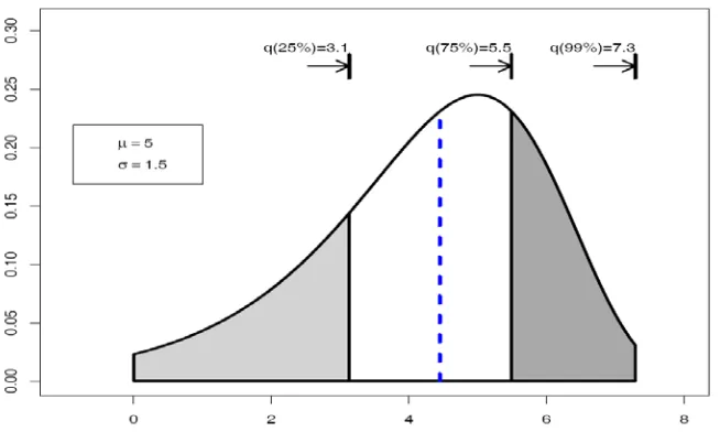
We developed the R function qlog.weibull ( ) for the computation of quantiles shown in Figure 3.
Fig. 3: Quantiles plots of the
LW(μ,σ)for
μ=5 and
σ=1.5vertical line indicates the median.
www.ijiset.com
function and the fitted distribution function when the parameters are obtained by method of maximum likelihood. The following graphical methods are used for suitability of the model under consideration, i.e., Quantile-Quantile(Q-Q) plot and Probability –Probability(P-P) plot.
3. Maximum Likelihood Estimation(MLE) and Information Matrix
For completeness purposes, we briefly discuss the maximum likelihood estimators (MLE’s) of the two-parameter LW(μ,σ) model and discuss their asymptotic properties to obtain approximate confidence intervals based on MLE’s[15].
Let x=(xR1R, . . . , xRnR) be a random sample of size n from LW(μ,σ), then the log-likelihood function can be written as;
n n
i i
i 1 i 1
x x
L( , ) n log exp
= =
− µ − µ
µ σ = − σ +∑ σ − ∑ σ
(10)
Therefore, to obtain the MLE’s of μ and σ, we can maximize (10) directly with respect to µ and σ or we can solve the following two non-linear equations:
n n n
i i i
2 i 1 i 1 i 1
x x x
L n 1
exp . 0
= = =
− µ − µ − µ
∂ = − − + =
∑ ∑ ∑
∂σ σ σ σ σ σ (11)
n i
i 1 x
L n 1
exp 0 = − µ ∂ = − + = ∑
∂µ σ σ σ (12)
Let us denote the parameter vector by θ = µ σ
(
,)
and the corresponding MLE of θ as θ = µ σˆ(
ˆ ˆ,)
then theasymptotic normality results in
( )
(
(
)
1)
2ˆ N 0, I( ) −
θ − θ → θ (13)
where I(θ) is the Fisher’s information matrix given by
2 2
2
2 2
2
ln L ln L
E E
I( )
L ln L
E E ∂ ∂ ∂µ ∂σ ∂µ θ = − ∂ ∂ ∂µ ∂σ ∂σ (14)
In practice, it is useless that the MLE has asymptotic variance
(
I( )θ)
−1because we do not know θ. Hence, we approximate the asymptotic variance by “plugging in” the estimated value of the parameters. The common procedure is to use observed Fisher information matrix O( )θˆ (as an estimate of the information matrix I(θ) given by2 2 2 ˆ 2 2 2 ˆ ˆ ( , )
ln L ln L
ˆ
O( ) H( )
ln L ln L θ=θ
µ σ ∂ ∂ ∂µ ∂σ ∂µ θ = − = − θ ∂ ∂ ∂µ ∂σ ∂σ (15)
where H is the Hessian matrix, θ=(μ,σ) and θˆ= ( , )µ σˆ ˆ . The Newton-Raphson algorithm to maximize the likelihood produces the observed information matrix. Therefore, the variance-covariance matrix is given by
(
)
1ˆ
ˆ ˆ ˆ
Var( ) cov( , ) H( )
ˆ ˆ ˆ
cov( , ) Var( ) − θ=θ µ µ σ − θ = µ σ σ
(16)
Hence, from the asymptotic normality of MLEs, approximate 100(1-γ)% confidence intervals for µ and σ can be constructed as
/2
ˆ zγ Var( )ˆ
µ ± µ and σ ±ˆ zγ/2 Var( )σˆ (17)
www.ijiset.com
For Computation of Maximum likelihood(ML) estimation, the following real data set is considered for illustration of the proposed methodology: Complete Data-Failure Times of 20 Components[11].
0.481, 1.196, 1.438, 1.797, 1.811, 1.831, 1.885, 2.104, 2.133, 2.144, 2.282, 2.322, 2.334, 2.341, 2.428, 2.447, 2.511, 2.593, 2.715, 3.218
The direct maximization of log-likelihood function given in (10) using Newton-Raphson method in R gives, the ML estimates and standard error. The 95% confidence interval is computed using (13) and (14). The Table 1 shows the ML estimates, standard error(SE) and 95 % Confidence Intervals parameters mu and sigma
Table 1: Maximum likelihood estimate, standard error and 95% confidence interval
Parameter MLE Std. Error 95% Confidence Interval
mu 2.36573 0.11674 (2.13691, 2.59455)
sigma 0.49441 0.08094 (0.33576, 0.65305)
4. Model Validation
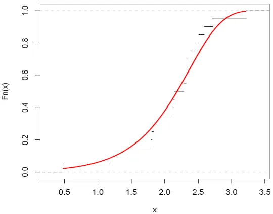
To check the validity of the model, we compute the Kolmogorov-Smirnov (KS) distance between the empirical distribution function and the fitted distribution function when the parameters are obtained by method of maximum likelihood. For this we developed R function ks.log.weibull( ). The result is presented in Table 3 and graph plots in Figure 4 which shows that the estimated Log-Weibull model provides excellent good fit to the given data[17].
Fig 4: The graph of empirical distribution function and fitted distribution function.
Let ˆF(x) be an estimate of F(x) based on xRlR, xR2R,. . . , xRnR. The scatter plot of the points
1 1:n
ˆF (p )− versus xRi : n R, i = 1 , 2, . . . ,n , is called a Q-Q plot which are another graphical method widely used for checking whether a fitted model is in agreement with the data. Thus, the Q-Q plots show the estimated versus the observed quantiles. If the model fits the data well, the pattern of points on the Q-Q plot will exhibit a 45-degree straight line. Note that all the points of a Q-Q plot are inside the square
[
]
1 1
1:n n:n 1:n n:n
ˆ ˆ
F− (p ) , F− (p ) x , x
×
www.ijiset.com
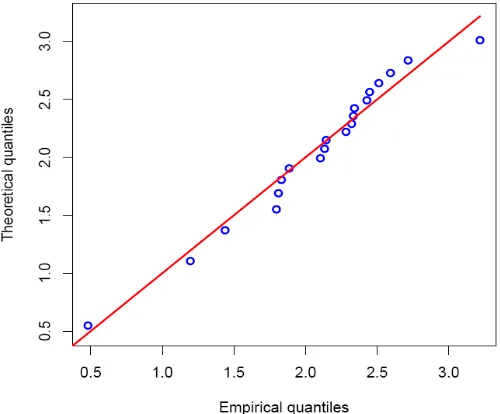
The corresponding R function qq.log.weibull() has developed. As can be seen from the straight line pattern in Figure 5 the Log-Weibull fits the data very well.
Fig 5: Quantile-Quantile(Q-Q) plot using MLEs as estimate.
5. Bayesian Estimation of Parameters of from LW(
μ,σ) by using of module akslog.weib(mu, sigma)
The developed module is implemented to obtain the Bayes estimates of the Log-Weibull model using MCMC method. The main function of the module is to generate MCMC sample from posterior distribution for Uniform prior.
It frequently happens that the experimenter knows in advance that the probable values of θ lie over a finite range [a, b] but has no strong opinion about any subset of values over this range. In such a case a uniform distribution over [a, b] may be a good approximation of the prior distribution, its p.d.f. is given by
1
; 0<a b
( ) b a
0 ; otherwise
≤ θ ≤
π θ = −
Bayesian Analysis with Uniform Priors as under:
A module akslog.weib(mu, sigma) is written in component Pascal, enables to perform full Bayesian analysis of Log-Weibull model into OpenBUGS using the method described in [18].The code contains three parts: model, data, and initial values.
Model {
for( i in 1 : N ) {
x[i] ~ akslog.weib(mu, sigma) }
# Prior distributions of the Model parameters mu ~ dunif(0.01, 10.0)
sigma~ dunif(0.01, 2.0) }
U
Data SetU
list(N=20, x=c(0.481, 1.196, 1.438, 1.797, 1.811, 1.831, 1.885, 2.104, 2.133, 2.144, 2.282, 2.322, 2.334, 2.341, 2.428, 2.447, 2.511, 2.593, 2.715, 3.218))
www.ijiset.com # Chain1
list(mu=1.0, sigma=0.1)
# Chain2
list(mu=5.0, sigma=1.2)
We run the model to generate two Markov Chains at the length of 40,000 with different starting points of the parameters. The convergence is monitored using trace and ergodic mean plots, we find that the Markov Chain converge together after approximately 2000 observations. Therefore, burnin of 5000 samples is more than enough to erase the effect of starting point(initial values). Finally, samples of size 7000 are formed from the posterior by picking up equally spaced every fifth outcome, i.e. thin=5, starting from 5001.This is done to minimize the auto correlation among the generated deviates.
Therefore, we have the posterior sample {μR1iR ,σR1iR}, i = 1,…,7000 from chain 1 and {μR2iR ,σR 2iR}, i = 1,…,7000 from chain 2.
The chain 1 is considered for convergence diagnostics plots. The visual summary is based on posterior sample obtained from chain 2 whereas the numerical summary is presented for both the chains.
5.1 Convergence diagnostics
The sequential realization of the parameters of the model gives an idea of the behavior of Morkov chain. The sequential realization of the parameters of the model is depicted in Fig 6.
History(Trace) plot
Fig 6: Sequential realization of the parameters μ and σ.
From the graph, we can conclude that the chain has converged as the plots show no long upward or downward trends, but look like a horizontal band.
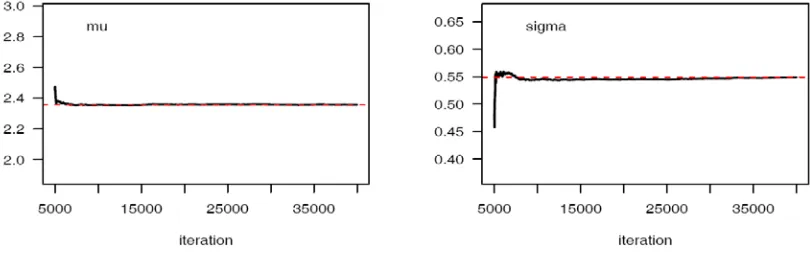
Running Mean (Ergodic mean) Plot
The convergence pattern can be studied by calculating the running mean which is the mean of all sampled values up to and including that at a given iteration. We thus generate a time series(Iteration number) graph of the running mean for each parameter in the chain. The Ergodic mean plots for the parameters shown in Figure 7 depict the convergence pattern.
www.ijiset.com Autocorrelation :
The graph shows that the correlation is almost negligible. We may conclude that the samples are independent.
Fig 8: The autocorrelation plots for mu and sigma.
5.2 Numerical Summary
The posterior is the ultimate experimental summary for a Bayesian. The location measures (especially the mean) of the posterior are of importance. The posterior mean represents Bayes estimator of the parameter under squared error loss function. The posterior mode and median are also Bayes estimators under different loss functions[16].
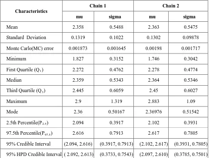
Table 2 : Numerical summaries based on MCMC sample of posterior characteristics for LW(μ,σ)
Characteristics
Chain 1 Chain 2
mu sigma mu sigma
Mean 2.358 0.5488 2.363 0.5475
Standard Deviation 0.1319 0.1022 0.1302 0.09878
Monte Carlo(MC) error 0.001873 0.001645 0.00198 0.001717
Minimum 1.827 0.3152 1.746 0.3042
First Quartile (QR1R) 2.272 0.4762 2.278 0.4774
Median 2.359 0.5343 2.364 0.5346
Third Quartile (QR3R) 2.445 0.6059 2.45 0.6027
Maximum 2.9 1.319 2.883 1.09
Mode 2.36 0.50167 2.36976 0.51542
2.5th Percentile(PR2.5R) 2.094 0.3917 2.102 0.3931
97.5th Percentile(PR97.5R) 2.616 0.7913 2.617 0.7805
95% Credible Interval (2.094, 2.616) (0.3917, 0.7913) (2.102, 2.617) (0.3931, 0.7805)
www.ijiset.com
5.3 Visual summary
Box plot
The boxes represent inter-quartile ranges and the solid black line at the (approximate) centre of each box is the mean; the arms of each box extend to cover the central 95 per cent of the distribution - their ends correspond, therefore, to the 2.5% and 97.5% quantiles. (Note that this representation differs somewhat from the traditional.)
Fig 9: The boxplots for mu and sigma
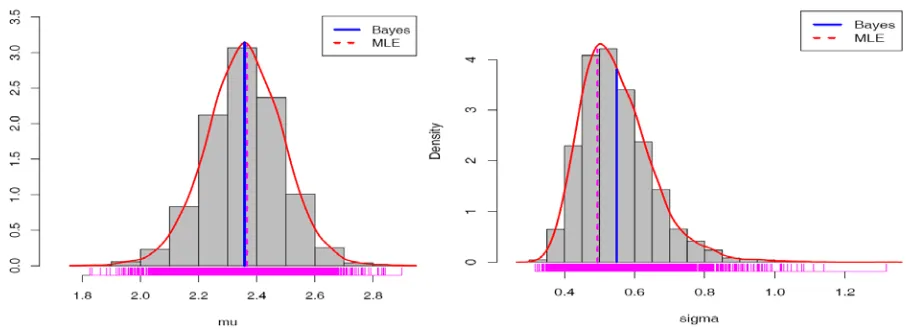
Kernel density estimates
Histograms can provide insights on skewness behavior in the tails, presence of multi-modal behaviour, and data outliers; histograms can be compared to the fundamental shapes associated with standard analytic distributions.
www.ijiset.com
Figure 10 provide the kernel density estimate of μ and σ. The kernel density estimates have been drawn using R with the assumption of Gaussian kernel and properly chosen values of the bandwidths. It can be seen that μ is symmetric whereas σ shows positive skewness.
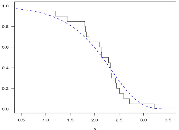
5.4 Comparison with MLE
For the comparison with MLE we have plotted three graphs. In Figure 11, the density functions f(x; , )µ σˆ ˆ using MLEs and Bayesian estimates, computed via MCMC samples under uniform priors, are plotted. The Figure 12 exhibits the estimated reliability function(dashed line) using Bayes estimate under uniform priors and the empirical reliability function(solid line). It is clear from the Figures, the MLEs and the Bayes estimates with respect to the uniform priors are quite close and fit the data very well.
Fig 11: Graphs of the density functions
f(x; , )
µ σ
ˆ ˆ
using MLEs and Bayesian estimates, computed via MCMC sampleswww.ijiset.com
6. Model Selection
Model selection encompasses many aspects. There are a number of distributions useful for modeling reliability data. For example, for analyzing failure times, most applications choose from the exponential, Weibull, or lognormal models. Consequently, one aspect of model selection is choosing a model for the reliability data. We present three general model selection methods.
Akaike information criterion (AIC).
AIC is defined as
AIC = - 2 loglikelihood (θˆ)+ 2 p
where θˆ is an estimate of θ and p is the number of parameters estimated in the model. The smaller the value of AIC the better the model
Bayesian information criterion (BIC)
Schwarz [13] proposed the Bayesian information criterion as
BIC = - 2 loglikelihood(θˆ) + p log(n)
where θˆ is an estimate of θ and p is the number of parameters estimated in the model. BIC is defined such that the smaller the value of BIC the better the model. For the computation of values of AIC and BIC we develop R function abic.log.weibull( ) .
Deviance information criterion (DIC)
The DIC is as a Bayesian counterpart to the AIC for model selection. One advantage is that the DIC can be calculated directly in OpenBUGS from the chains produced by an MCMC run. Model with smaller DIC is taken to be better. The values are DIC are computed in OpenBUGS where pD stands for effective number of parameters.
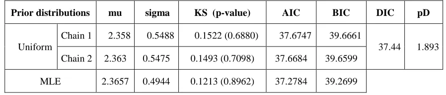
The Table 3 shows the values of different information measures(AIC, BIC and DIC) and Kolmogorov-Smirnov(K-S) distance. The ‘plug-in’ values of AIC and BIC for Bayes estimates.
Table 3: Different information measures(AIC, BIC and DIC) and K-S distance
Prior distributions mu sigma KS (p-value) AIC BIC DIC pD
Uniform
Chain 1 2.358 0.5488 0.1522 (0.6880) 37.6747 39.6661
37.44 1.893 Chain 2 2.363 0.5475 0.1493 (0.7098) 37.6684 39.6599
MLE 2.3657 0.4944 0.1213 (0.8962) 37.2784 39.2699
7. Conclusion
The Log-Weibull model with shape parameter µ and scale parameter σ has been discussed and estimate of its parameters obtained based on a complete sample by using the Markov chain Monte Carlo (MCMC) method. The MCMC method has proven more effective as compared to the usual methods of estimation.
www.ijiset.com
Acknowledgments
The authors are thankful to the editor and the referees for their valuable suggestions, which improved the paper to a great extent.
References
[1]. Christopeit, N. (1994). Estimating parameters of an extreme value distribution by the method of moments, Journal of Statistical Planning and Inference, 41, 173–186
[2]. Dekkers, A.L., Einmahl, J.H.J. and De Haan, L. (1989). A moment estimator for the index of an extreme–value distribution, Annals of Statistics, 17, 1833–1855
[3]. Johnson, N. L., Kotz, S., and Balakrishnan, N. (1994). Continuous Univariate Distributions-1, 2nd edition. John Wiley and Sons, New York.
[4]. Johnson, N. L., Kotz, S., and Balakrishnan, N. (1995). Continuous Univariate Distributions-2, 2nd edition. John Wiley and Sons, New York.
[5]. Klugman, S., Panjer, H. and Willmot, G. (2004) Loss Models: From Data to Decisions, 2nd ed.,New York, Wiley. [6]. Kotz, S. and Nadarajah S. (2000). Extreme Value Distributions:Theory and Applications, Imperial College Press, London. [7]. Kotz, S., Balakrishnan, N. & Johnson, N.L., 2000. Continuous Multivariate Distributions, Volume 1, Models and Applications,
2nd Edition 2nd ed., Wiley-Interscience.
[8]. Lieblein, J. and Zelen, M. (1956). Statistical investigation of the fatigue life of ball bearings, Journal of Research of National Bureau of Standards, 57, 273–315.
[9]. Lyu M.R., (1996). Handbook of Software Reliability Engineering, IEEE Computer Society Press, McGraw Hill, 1996. [10].Marshall, A. W., Olkin, I.(2007). Life Distributions: Structure of Nonparametric, Semiparametric, and Parametric Families,
Springer, New York.
[11].Murthy, D.N.P., Xie, M., Jiang, R. (2004). Weibull Models, Wiley, New Jersey. [12].Rinne, H., 2008. The Weibull Distribution: A Handbook 1st ed., Chapman & Hall/CRC. [13].Schwarz, G. (1978). Estimating the dimension of a model. The Annals of Statistics, 6, 461–464.
[14].Singpurwalla, N.D. and S. Wilson (1994). Software Reliability Modeling. International Statist. Rev., 62 3:289-317.
[15].Srivastava, A.K. and Kumar, V.(2011). “Analysis of Pham(Loglog) Reliability Model using Bayesian Approach”, International Journal ‘Computer Science Journal’, Vol. 1(2),79-100, ISSN: 2221–5905.
[16].Srivastava, A.K. and Kumar, V.(2011). “Markov Chain Monte Carlo Methods for Bayesian Inference of the Chen Model”, International Journal of Computer Information Systems, Vol. 2(2), 07-14, ISSN: 2229-5208.
[17].Srivastava, A.K. and Kumar, V.(2015). “ A study on several issues of Reliability Modelling for a Real Data Set using different Software Reliability Models”, International Journal of Emerging Technology and Advanced Engineering, Vol.05(12), 49-57, ISSN: 2250 - 2459.
[18].Thomas, A. (2010). OpenBUGS Developer Manual, Version 3.1.2, http://www.openbugs.info/.