Evolutionary deep learning

(1)

University

of

Cape

Town

Author:

Emmanuel DUFOURQ

Supervisor:

Prof. Bruce A. BASSETT

Thesis Presented for the Degree of

Doctor of Philosophy

in the

Department of Mathematics and Applied Mathematics

University of Cape Town

and

African Institute for Mathematical Sciences

(2)

University

of

Cape

Town

The copyright of this thesis vests in the author. No

quotation from it or information derived from it is to be

published without full acknowledgement of the source.

The thesis is to be used for private study or

non-commercial research purposes only.

Published by the University of Cape Town (UCT) in terms

of the non-exclusive license granted to UCT by the author.

(3)

Declaration of Authorship

I, Emmanuel DUFOURQ, declare that this thesis titled, “Evolutionary Deep Learning” and the work presented in it are my own. I confirm that:

• This work was done wholly or mainly while in candidature for a re-search degree at this University.

• Where any part of this thesis has previously been submitted for a de-gree or any other qualification at this University or any other institu-tion, this has been clearly stated.

• Where I have consulted the published work of others, this is always clearly attributed.

• Where I have quoted from the work of others, the source is always given. With the exception of such quotations, this thesis is entirely my own work.

• I have acknowledged all main sources of help.

• Where the thesis is based on work done by myself jointly with others, I have made clear exactly what was done by others and what I have contributed myself.

Signed:

(4)

Declaration of Publications

• Publication 1 Dufourq, E., Bassett, B. A., Automated Classification of Text Sentiment, SAICSIT 2017, South Africa. Presented in chapter4.1in this thesis.

• Publication 2 Dufourq, E., Bassett, B. A., Automated Problem Identifi-cation: Regression vs Classification via Evolutionary Deep Networks, SAICSIT 2017, South Africa. Presented in chapter5in this thesis.

• Publication 3 Dufourq, E., Bassett, B. A., Text Compression for Senti-ment Analysis via Evolutionary Algorithms, PRASA-ROBMECH 2017, South Africa. Presented in chapter6in this thesis.

• Publication 4 Dufourq, E., Bassett, B. A., EDEN: Evolutionary Deep Networks for Efficient Machine Learning, PRASA-ROBMECH 2017, South Africa. Presented in chapter4in this thesis.

(5)

Evolutionary Deep Learning

by Emmanuel DUFOURQ

The primary objective of this thesis is to investigate whether evolutionary concepts can improve the performance, speed and convenience of algorithms in various active areas of machine learning research.

Deep neural networks are exhibiting an explosion in the number of pa-rameters that need to be trained, as well as the number of permutations of possible network architectures and hyper-parameters. There is little guid-ance on how to choose these and brute-force experimentation is prohibitively time consuming. We show that evolutionary algorithms can help tame this explosion of freedom, by developing an algorithm that robustly evolves near-optimal deep neural network architectures and hyper-parameters across a wide range of image and sentiment classification problems. We further de-velop an algorithm that automatically determines whether a given data sci-ence problem is of classification or regression type, successfully choosing the correct problem type with more than 95% accuracy. Together these al-gorithms show that a great deal of the current "art" in the design of deep learning networks - and in the job of the data scientist - can be automated.

Having discussed the general problem of optimising deep learning net-works the thesis moves on to a specific application: the automated extraction of human sentiment from text and images of human faces. Our results re-veal that our approach is able to outperform several public and/or commer-cial text sentiment analysis algorithms using an evolutionary algorithm that learned to encode and extend sentiment lexicons. A second analysis looked at using evolutionary algorithms to estimate text sentiment while simulta-neously compressing text data. An extensive analysis of twelve sentiment datasets reveal that accurate compression is possible with 3.3% loss in classi-fication accuracy even with 75% compression of text size, which is useful in environments where data volumes are a problem.

Finally, the thesis presents improvements to automated sentiment anal-ysis of human faces to identify emotion, an area where there has been a tremendous amount of progress using convolutional neural networks. We provide a comprehensive critique of past work, highlight recommendations and list some open, unanswered questions in facial expression recognition

(6)

using convolutional neural networks. One serious challenge when imple-menting such networks for facial expression recognition is the large number of trainable parameters which results in long training times. We propose a novel method based on evolutionary algorithms, to reduce the number of trainable parameters whilst simultaneously retaining classification perfor-mance, and in some cases achieving superior performance.

We are robustly able to reduce the number of parameters on average by 95% with no loss in classification accuracy. Overall our analyses show that evolutionary algorithms are a valuable addition to machine learning in the deep learning era: automating, compressing and/or improving results sig-nificantly, depending on the desired goal.

(7)

Many thanks to my supervisor, Professor Bruce Bassett, for his invaluable guidance, encouragement, support and words of extreme wisdom through-out this degree. He has been an incredible mentor and friend.

A million thanks to my parents for their daily support, for listening to every single detail I had to say in each conversation, for providing me with guidance, and continuous love and encouragement from the first day. A spe-cial thanks to Lauren for her infinite kindness, love and support.

Many thanks to the staff and Cosmology group at the African Institute for Mathematical Sciences. Thanks for welcoming me and providing a great working environment. Thanks to Martin Kunz to granting access to the Baobab cluster at the University of Geneva.

I would also like to thank the following people who have helped me or impacted my research in a positive way throughout this degree: Shankar Agarwal, Etienne Vos, Ethan Roberts, Michelle Lochner, Dee Knights, Pierre-Yves Lablanche, Nadeem Oozeer, Kimeel Sooknunan, Louwrens Labuschagne, Blake Cuningham, Yabebal Tadesse, Kayode Olaleye, Matthew Nixon, Mark Heerden, Arun Aniyan, Ian Durbach, Bubacarr Bah, Zafiirah Hosenie, Alireza Sadr, Kai Stats, Arrykrishna Mootoovaloo, Gilad Amar, Diego Cardenas, Anne and Mark Pennels, James and Karen Barnes, and Rene January.

The financial assistance of the National Research Foundation (NRF) to-wards this research is hereby acknowledged. Opinions expressed and con-clusions arrived at, are those of the authors and are not necessarily to be attributed to the NRF.

(8)

List of Figures

2.1 Timeline illustrating selected significant advances in machine

learning from the 1950’s to the present.. . . 10

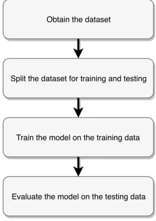
2.2 Primary steps involved when implementing a machine learn-ing algorithm. . . 12

2.3 Highlighting the primary components related to the dataset terminology. . . 13

2.4 Illustrating 10-fold cross-validation. . . 14

2.5 Illustrating how a dataset is split into training, validation and testing sets.. . . 15

2.6 Illustrating two evolutionary algorithm representations. . . . 19

2.7 Illustrating tournament parent selection. . . 22

2.8 Illustrating the reproduction genetic operator. . . 23

2.9 Illustrating the mutation genetic operator. . . 24

2.10 Illustrating the crossover genetic operator. . . 25

2.11 Illustrating the evolutionary process. . . 26

2.12 Illustrating the analogy that neural networks takes from neu-roscience. . . 27

2.13 Illustrating a perceptron single layer network. . . 28

2.14 Illustrating a 2 layer neural network. . . 30

2.15 Illustrating forward pass computations. . . 31

2.16 The effect of the learning rate. . . 32

2.17 Network to illustrate gradient descent . . . 33

2.18 Illustrating the oscillations that take place during gradient de-scent . . . 35

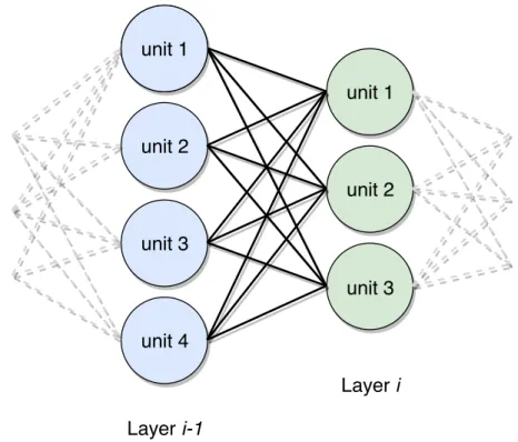
2.19 Illustrating a neural network with 3 layers. . . 36

2.20 Illustrating a fully connected layer. . . 37

2.21 Illustrating how convolutional layers are applied. . . 39

2.22 Illustrating the width and the height of the input image, the filter and the feature map. . . 39

2.23 Illustrating the spatial reduction achieved by performing max pooling.. . . 40

(14)

3.1 Example of a network architecture generated by anAPI

chro-mosome. . . 46

3.2 API chromosome which encodes the categorical cross entropy error loss function, . . . 46

3.3 Illustrating fitness calculation. . . 51

3.4 APImutation operator. . . 53

3.5 APIcrossover operator. . . 53

3.6 Accuracy (%) results obtained byAPIon the various datasets. 57 4.1 Illustrates an example of a neural network evolved using EDENfor sentiment analysis. . . 65

4.2 An example of anEDENchromosome. . . 67

4.3 An example of the embedding operation. . . 68

4.4 Illustrating the replacement mutation operator. . . 69

4.5 Illustrating the addition mutation operator. . . 71

4.6 Illustrating the delete mutation operator. . . 72

4.7 Change in mean fitness over the GA generations for the MNIST data. . . 76

4.8 Change in mean learning rate over the GA generations. . . 77

5.1 Example of aGASAchromosome.. . . 83

5.2 Example ofGASAmutation. . . 86

5.3 Example ofGASAcrossover. . . 87

5.4 Example of aCA-GASAchromosome. . . 97

6.1 An example of a PARSEC compressor with 10 rules. . . 104

6.2 Illustrating how PARSEC compresses text.. . . 105

6.3 Change in average PARSEC test accuracy. . . 114

6.4 Illustrating four rules which were extracted from a PARSEC compressor. . . 115

7.1 A subject expressing surprise. . . 122

7.2 Flowchart illustrating the primary steps involved when imple-menting a CNN for FER. . . 124

7.3 Six common expressions found in the majority of the FER datasets. . . 127

7.4 Difference between images from “in the wild” datasets and laboratory posed datasets. . . 129

(15)

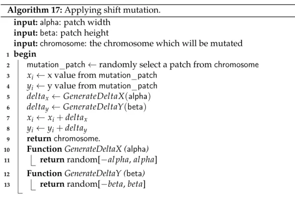
8.3 Illustrating shift and standard mutation . . . 151

8.4 EvoFER crossover operator. . . 153

8.5 Illustrating the EvoFER pipeline. . . 154

8.6 Different augmentation techniques which are used inEvoFER. 157

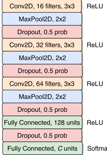
8.7 CNN architecture used in EvoFER experiment. . . 158

8.8 Patches extracted from the best chromosome on JAFFE dataset. 162

8.9 Patches extracted from the best chromosome on KDEF dataset. 163

8.10 Patches extracted from the best chromosome on MUG dataset. 163

8.11 Patches extracted from the best chromosome on RAFD dataset. 164

A.1 Illustrating image augmentation. . . 172

A.2 Difference between the two primary ensemble methods which were observed in the studies surveyed. . . 176

(16)

List of Tables

3.1 The 16 datasets used in theAPIstudy. . . 55

3.2 The GA parameters used in theAPIstudy.. . . 56

3.3 The neural network parameters used in theAPIstudy. . . 58

3.4 APIclassification results. . . 58

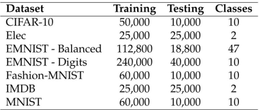
4.1 The datasets used in theEDENstudy. . . 74

4.2 The GA and neural network parameters used in theEDENstudy. 74 4.3 EDENtest accuracy (%) results. . . 75

4.4 Average training times, in hours, for a singleEDENexperiment. 75 5.1 Data sets used in theGASAstudy. . . 89

5.2 GASAparameters used in the study. . . 89

5.3 Test accuracy (%) results on the two class review problem (sen-timent and amplifier). . . 91

5.4 Test accuracy (%) results on the two class summary problem (sentiment and amplifier). . . 91

5.5 Test accuracy (%) results on the two class problem review (pos-itive and negative sentiment) . . . 92

5.6 Test accuracy (%) results on the two class combined problem (positive and negative sentiment) . . . 93

5.7 ComparingGASAto other algorithms. . . 94

5.8 ComparingGASAandCA-GASA.. . . 97

6.1 Common parts-of-speech. . . 103

6.2 The lower and upper compression bound constrain. . . 111

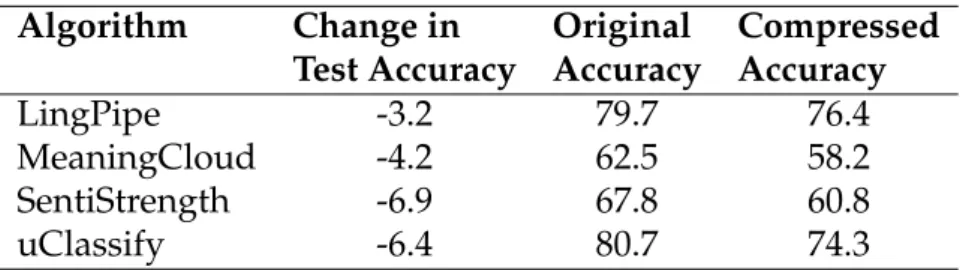
6.3 Average change inPARSECtest accuracy (%) . . . 113

6.4 Difference in performance with 10% compression rate. . . 117

(17)

a CNN for FER. . . 125

7.2 Characteristics of the most commonly used FER datasets. . . . 126

7.3 Various network architectures reported in the studies surveyed.134

7.4 Average, standard deviation, minimum and maximum of the

CNN architectures used in the studies surveyed. . . 137

7.5 Activation functions that were reported in the studies

sur-veyed that implemented their own CNN architecture. . . 137

7.6 Classification accuracy results (%) on the CK+ dataset. . . 142

7.7 Classification accuracy results (%) on the JAFFE dataset. . . . 142

7.8 Classification accuracy results (%) on the FER’13 dataset. . . . 143

7.9 Classification accuracy results (%) on the EmotiW’17 dataset.. 143

7.10 Classification accuracy results (%) on the SFEW dataset. . . 143

7.11 Classification accuracy results (%) on the KDEF dataset. . . 144

8.1 Number of training images used in theEvoFERstudy for each

dataset after the images were augmented. . . 156

8.2 Parameters associated with the evolutionary algorithm in the

EvoFERstudy. . . 159

8.3 Parameters associated with the CNN in theEvoFERstudy. . . 159

8.4 Additional parameters used in theEvoFERstudy. . . 159

8.5 Test classification accuracy (%) for the CNN network on the

original images and performance when usingEvoFER. . . 160

8.6 The average number of trainable neural network parameters

when using the original image andEvoFERextracted patches. 161

8.7 Average time taken (seconds) to process 10 images using

EvoFERand the baseline CNN architecture. . . 164

A.1 Commonly used data augmentation techniques. . . 172

A.2 Deep learning frameworks which were used in the studies sur-veyed.. . . 175

(18)

(19)

Chapter 1

Introduction

Progress in machine learning [177] has skyrocketed over recent years. Ma-chine learning has been applied to a vast number of domains such as product recommendations, social media analysis, search engines, face identification and emotion analysis. Machine learning is transforming academic research by enabling researchers to gain insights into problems which would take hu-mans a great amount of time. This transformation is also noticeable in indus-try where machine learning is being used to automate challenging tasks. The number of research articles published on machine learning has also drasti-cally increased especially with the undeniable attention that deep learning [138,229,85] has received.

Amongst the large number of machine learning algorithms which have been proposed over the years is one which has been inspired by biological evolution. Just as Leonardo da Vinci and the Wright brothers studied the flight of birds to enable their works on creating a flying machine [219, 102], researchers have turned to nature to develop evolutionary computational methods (which use natural selection to blend and evolve a population of candidate solutions to find an optimal or near-optimal solution) [15, 270,69,

14] to enable them to solve optimisation problems.

1.1

Purpose of the Study

The primary objective of this thesis is to investigate how evolutionary ma-chine learning can be adapted and applied to various active areas of research. Based on literature surveys, we explore and investigate the modifications necessary to address these areas which have not previously been researched. The focus was not to investigate on how to create new state-of-the-art ap-proaches, but rather to evaluate and investigate novel approaches. We for-mulate the following six objectives for this thesis.

(20)

1. Does the problem require estimating a continuous value (regression) or a discrete class label (classification)? This is perhaps the most ba-sic question faced when tackling a new supervised learning problem. Humans are able to study a dataset and decide whether it represents a classification or a regression problem, and consequently make deci-sions which will be applied to the execution of a neural network. The objective is to propose a machine learning algorithm that can automat-ically identify the problem type with the aim of moving towards algo-rithms that are more intelligent. The proposed method will be applied to various classification and regression datasets.

2. Deep neural networks continue to show improved performance with increasing depth, an encouraging trend that implies an explosion in the possible permutations of network architectures and hyper-parameters for which there is little intuitive guidance. Following from the previ-ous objective, we propose to investigate how an evolutionary algorithm can be applied to optimise neural network architectures and associated hyper-parameters. The proposed method will be investigated by ex-perimenting on various problem types such as natural language pro-cessing and computer vision problems.

3. For adult humans, interpreting the underlying emotions in text is usu-ally performed unconsciously and with apparent ease. We are able to recognize emotions in emails, sentiments in our social media feed and appreciate the subtle nuances of conflicting views in novels. Neverthe-less, even for humans text can be notoriously easy to misinterpret. For machines, on the other hand, sentiment analysis is highly non-trivial. The objective is to propose and investigate how an evolutionary algo-rithm can be applied to this problem domain. The proposed approach will be evaluated on a number of text sentiment datasets.

4. Following the previous objective, we pose the following question, can textual data be compressed intelligently without losing accuracy in evaluating sentiment? There are often a large number of redundant words which humans use when expressing their sentiment about some-thing. The objective is to propose an evolutionary algorithm which can compress text in such as way that the classification accuracy is not sig-nificantly impacted. The proposed approach will be evaluated on a number of text sentiment datasets.

(21)

tional neural networks for facial expression recognition. We propose as an objective, to provide a critical analysis of works using convo-lutional neural networks for facial expression recognition. The anal-ysis should enable researchers who are new to the field to rapidly gain knowledge as to different available approaches. Furthermore, the ob-jective is to provide established researchers with unanswered questions which need addressing.

6. One challenge when implementing convolutional neural networks for facial expression recognition is the large number of trainable parame-ters. This can result in large training times and the inability to train deep networks on limited hardware. Following the previous objective, we propose to investigate how evolutionary machine learning can be incorporated with convolutional neural networks in order to achieve good predictive performance while simultaneously reducing the num-ber of trainable parameters. The proposed approach will be evaluated on various facial expression recognition datasets.

1.2

Contributions

This thesis makes the following contributions:

1. Experimenters and researchers make a lot of decisions when imple-menting neural networks. For example, when creating deep neural networks, the number of parameters must be selected in advance and furthermore, a lot of these choices are made based upon pre-existing knowledge of the data such as the use of a categorical cross entropy loss function. Humans are able to study a dataset and decide whether it represents a classification or a regression problem, and consequently make decisions which will be applied to the execution of the neural network. There have not been any previous attempts to propose an al-gorithm that can automatically discriminate between classification and regression problems and to automatically decide on the loss function and number of units in the last layer of a neural network. We propose the Automated Problem Identification (API) algorithm, which uses an evolutionary algorithm interface to TensorFlow to manipulate a deep neural network to decide if a dataset represents a classification or a

(22)

regression problem. We test API on 16 different classification, regres-sion and sentiment analysis datasets with up to 10,000 features and up to 17,000 unique target values. API achieves an average accuracy of 96.3% in identifying the problem type without hardcoding any in-sights about the general characteristics of regression or classification problems. These findings are revealed in chapter4.1.

2. Following the previous contribution, we examined how to adapt an evolutionary algorithm to enable the automatic creation of deep neural networks. We propose Evolutionary DEep Networks (EDEN), a com-putationally efficient neuro-evolutionary algorithm which interfaces to any deep neural network platform, such as TensorFlow. We show that EDEN evolves simple yet successful architectures built from embed-ding, 1D and 2D convolutional, max pooling and fully connected layers along with their hyper-parameters. Evaluation of EDEN across seven image and sentiment classification datasets shows that it reliably finds good networks – and in three cases achieves state-of-the-art results – even on a single GPU, in just 6-24 hours. Our study provides a first at-tempt at applying neuro-evolution to the creation of 1D convolutional networks for sentiment analysis including the optimisation of the em-bedding layer. These findings are revealed in chapter4.

3. The ability to identify sentiment in text, referred to as sentiment anal-ysis, is one which is natural to adult humans. This task, however, is not one which a computer can perform by default. Identifying senti-ments in an automated, algorithmic manner will be a useful capabil-ity for business and research in their search to understand what con-sumers think about their products or services and to understand hu-man sociology. Here we propose two new genetic algorithms for the task of automated text sentiment analysis. The genetic algorithms learn whether words occurring in a text corpus are either sentiment or am-plifier words, and their corresponding magnitude. Sentiment words, such as ’horrible’, adds linearly to the final sentiment. Amplifier words in contrast, which are typically adjectives/adverbs such as ’very’, mul-tiply the sentiment of the following word. This increases, decreases or negates the sentiment of the following word. The sentiment of the full text is then the sum of these terms. This approach grows both a senti-ment and amplifier dictionary which can be reused for other purposes and fed into other machine learning algorithms. We report the results

(23)

sults reveal that our proposed approach was able to outperform several public and/or commercial sentiment analysis algorithms. These find-ings are revealed in chapter5.

4. Text reviews are often lengthy and contain a lot of extra words which do not contribute to the sentiment which is being expressed by the au-thor. We propose a novel evolutionary compression algorithm, PAR-SEC (PARts-of-Speech for sEntiment Compression), which makes use of Parts-of-Speech tags to compress text in a way that sacrifices minimal classification accuracy when used in conjunction with sentiment analy-sis algorithms. An analyanaly-sis of PARSEC with eight commercial and non-commercial sentiment analysis algorithms on twelve English sentiment data sets reveals that accurate compression is possible with (0%, 1.3%, 3.3%) loss in sentiment classification accuracy for (20%, 50%, 75%) data compression with PARSEC using LingPipe, the most accurate of the sentiment algorithms. Other sentiment analysis algorithms are more severely affected by compression. We conclude that significant com-pression of text data is possible for sentiment analysis depending on the accuracy demands of the specific application and the specific sen-timent analysis algorithm used. These findings are revealed in chapter

6.

5. Humans are generally good at recognising emotions which are por-trayed on another person’s face. Can the same be said for machines? In recent years, there has been a tremendous amount of progress in the field of computer vision using deep learning methods, namely by con-volutional neural networks. How good are these concon-volutional neural networks at recognising facial expressions? With the explosion of re-search outputs using convolutional neural networks for facial expres-sion recognition in recent years, it is an appropriate time to review the state of the art in this field, provide a critical analysis of what has and has not been achieved, and synthesize recommendations for each step of the process needed for facial expression recognition. This work serves as a guide to those who are new to the field. This survey pro-vides a critique of past work, highlights recommendations and lists some open, unanswered questions in facial expression recognition that deserve further investigation. The survey and analysis is presented in chapter7.

(24)

6. The previous objective dealt with reviewing studies that use convolu-tional neural networks for facial expression recognition. Convoluconvolu-tional neural networks are known to result in a large number of neural net-work parameters. Can these parameters be reduced intelligently in such a way as to preserve the predictive ability of the convolutional neural network? We propose and investigate an evolutionary algo-rithm for facial expression recognition. The proposed algoalgo-rithm ex-tracts patches from an image and trains the convolutional neural net-work on the patches instead of the entire face. The objective was to minimise the number of parameters and maximise the classification ac-curacy. We demonstrate that the algorithm can reduce the number of parameters on average by 95% and simultaneously increase the clas-sification accuracy. The method and findings are presented in chapter

8.

1.3

Thesis Layout

In this section we present the layout of the thesis and briefly describe the contents of each chapter.

Chapter 2 - Introduction to Machine Learning

The reader is introduced to machine learning. Supervised machine learning problems are typically either regression or classification problems. In this chapter we present the characteristics and discuss both classification and re-gression problems. We define the metrics which are used to evaluate such problems and introduce the reader to terminology used throughout the the-sis. The chapter then discusses evolutionary algorithms and presents the reader with the fundamental knowledge required to understand the method. The various aspects of the method are described in detail. Finally, the chapter introduces deep neural networks.

Chapter 3 - Neuro-evolutionary Problem Identification

Researchers and experimenters typically make certain premeditated deci-sions based on whether they are addressing a classification or regression problem. In this chapter we present a novel approach which enables an al-gorithm to automatically make these decisions using evolutionary machine learning.

(25)

When using a neural network one has to make a lot of decisions with regards to the architecture of the network and the associated hyper-parameters. In this chapter we present an evolutionary approach which attempts to optimise neural network architectures and the hyper-parameters.

Chapter 5 - Automated Classification of Text Sentiment

The ability to identify sentiment in text, referred to as sentiment analysis, is one which is natural to adult humans. In this chapter we propose an evolu-tionary algorithm for text sentiment analysis. We report the results of multi-ple experiments conducted on large Amazon data sets.

Chapter 6 - Text Compression for Sentiment Analysis via

Evo-lutionary Algorithms

Following the previous contribution, in this chapter, we propose a novel evo-lutionary compression algorithm which makes use of Parts-of-Speech tags to compress text in a way that sacrifices minimal classification accuracy when used in conjunction with sentiment analysis algorithms.

Chapter 7 - Facial Expression Recognition and Convolutional

Neural Networks

Humans are generally good at recognising emotions which are portrayed on another person’s face. With the explosion of research outputs using convo-lutional neural networks for facial expression recognition in recent studies, it is an appropriate time to review the state of the art in this field, provide a critical analysis of what has and has not been achieved, and synthesize recommendations for each step of the process needed for facial expression recognition.

(26)

Chapter 8 - Evolutionary Facial Expression Recognition

The previous chapter reviews studies that use convolutional neural networks for facial expression recognition. The review reveals that convolutional neu-ral networks achieve state-of-the-art performance as opposed to other ma-chine learning methods. In this chapter, we explore a novel idea which at-tempts to optimise the predictive performance of convolutional neural net-works for facial expression recognition and simultaneously, reduce the num-ber of trainable network parameters without compromising on the classifica-tion accuracy.

Chapter 9 - Conclusion

We conclude this thesis by providing a summary of the findings which were observed throughout the experiments conducted in the previous chapters. We highlight the objectives presented in the first chapter and discuss how these have been met. This chapter provides direction for future research.

(27)

Chapter 2

Introduction to Machine Learning

2.1

Introduction

This chapter introduces the reader to machine learning. The following sec-tion introduces the general idea and history of machine learning. Secsec-tion

2.3introduces various terminology and presents the reader with the primary steps to undertake when implementing a machine learning algorithm. An introduction to evolutionary algorithms is presented in section2.4 which is the fundamental technique used throughout this thesis. The various aspects of the evolutionary algorithm are discussed in detail. Section 2.5 provides an introduction to deep learning and equips the reader with the necessary knowledge for the methods implemented in this thesis. Finally, section 2.6

concludes this chapter.

2.2

Introduction to Machine Learning

Machine learningalgorithms deal with the creation of models which enable a computer program to recognise patterns, learn relationships between data, make predictions and mimic the brain’s ability to learn [177]. Mitchell [177] stated that “a computer program is said to learn from experienceEwith re-spect to some class of tasksTand performance measurePif its performance at tasks inT, as measured byP, improves with experienceE". Certain tasks, or problems are far too challenging and would take too long for a human to solve. Machine learning on the other hand has been used to solve a vast number of problems. For example, a large number of data classification tasks were solved using machine learning [126], more specifically using genetic programming in [65]. The performance measures are discussed in the fol-lowing subsections. The experience, E, can be supervised or unsupervised. In supervised machine learning the problems have input variables for which

(28)

the algorithm can be applied on to obtain output values. Unsupervised ma-chine learning refers to problems for which there are input variables but there are no output variables which need predicting. Here the machine learning al-gorithm learns useful properties of the structure of this dataset [85].

Early works in machine learning date back to 1950’s where Arthur Samuel [224] proposed and invented an algorithm which played the board game checkers. Since then several breakthroughs were made, notably when Deep-Blue [26] outperformed chess champion Garry Kasparov. LeCun [137] demonstrated that a machine learning algorithm, namely a convolutional neural network could learn how to recognise hand written digits in 1998. Neural networks gained significant attention in 2012 when they were used to win the ImageNet challenge where the task is to correctly identify images from a corpus of millions of images [130]. More recently, DeepMind pro-duced AlphaGo, a machine learning algorithm which outperformed grand-master Lee Sedol, a champion at the game of Go in 2016 [236]. Figure 2.1

highlights a number of selected advances in machine learning from the 1950’s to the present.

Present, 2018 1959 - Samuel proposed

a machine learning algorithm to play board

game checkers. 1996 - IBM's DeepBlue outperformed chess champion Garry Kasparov. 2016 - AlphaGo outperformed professional Go player. 2012 - ImageNet challenge winner used convolutional

neural network.

1998 - LeCun proposed a convolutional neural

network which can perform digit recognition.

2015 - DeepMind proposed DQN which achieves human

level performance on Atari Breakout game.

FIGURE2.1: Timeline illustrating selected significant advances in machine learning

(29)

to:

• sentiment analysis [193]

• assisting people with limited mobility [95]

• pneumonia detection [211]

• skin cancer classification [72]

Examples of machine learning algorithms include, but are not limited to:

• metaheuristics including evolutionary algorithms [22]

• neural networks [75]

• decision trees [127]

• support vector machines [43]

2.3

Applying Machine Learning

This section introduces various concepts and terminology associated with the implementation of machine learning algorithms. Figure 2.2 illustrates the steps which are performed in such implementations. These steps are ex-plained in further details in the subsections below.

2.3.1

Dataset terminology

The first step in implementing a machine learning algorithm is to acquire a dataset. Adatasetcan be defined as a collection of records which encode some information about a particular problem. Each record, or row in a dataset is referred to as anexampleorinstance. Thus, a dataset is made up of a number of examples. Each example in turn is made up of a number of features and often atarget. The features, or attributes denote the characteristics of the ex-amples and the target denotes the variable which must be predicted for each example [23]. Features can be discrete or continuous values. Thus, typically a dataset is made up of a number of examples and corresponding targets. There can be one or multiple features and, one or multiple targets. In clas-sification tasks the target is also referred to as theclass. A machine learning model is thus one which can map the input features to the targets [131]. In

(30)

Obtain the dataset

Split the dataset for training and testing

Train the model on the training data

Evaluate the model on the testing data

FIGURE2.2: Primary steps involved when implementing a machine learning algo-rithm. The steps exclude any pre-processing that needs to be done to the dataset and

hyper-parameter optimisation for the algorithm.

the case of a classification task the model is also referred to as the classifier. Figure2.3illustrates an example of a dataset which is made up of a number of examples. Each example has a number of features and a target.

2.3.2

Classification and Regression

In classification tasks the objective is to construct a model that can correctly predict the classes for as many examples as possible. A perfect classifier is one that correctly predicts all of the examples. The targets are discrete finite categories. Classification problems with two classes are referred to as binary classification, and if the problem has more than two then it is called multi-class multi-classification. On the other hand,regression problems have continuous values in the targets. For regression, the objective is to construct a model that can predict values as close as possible to the targets in each example. A perfect model for a regression problem is one that predicts the exact val-ues for all of the examples. Classification and regression problems are both supervised machine learning problems.

(31)

Feature 1 Feature 2 Feature 4 Feature 5

Example / instance

Dataset

Feature 3 Target

FIGURE2.3: Highlighting the primary components related to the dataset terminol-ogy. The dataset is represented by the whole table. Each row in the dataset is an example, for which the examples are made up of a number of features and targets. In the figure there are five features and one target. Each feature is represented as a

column, and the right most column is the target.

2.3.3

Data splitting

The dataset needs to be split so that a model can be evaluated and to deter-mine its performance. Typically, the dataset will be split in such a way that there is training data for which the model learns from – this is the training

phase. Furthermore, the dataset needs to be split in such a way that some of the data can be used to evaluate how the model is doing on data it has not seen before (i.e. an unbiased performance evaluation)[131] – this is the

testingphase. The unseen data is referred to as the test data. The test data is used to evaluate the trained model. Training a model and evaluating its per-formance on the same training data is not a true representation of the model as the model can be fit perfectly to the training data and thus achieve per-fect predictive ability on that data [280]. It is thus important that the training and testing data are disjoint sets [280]. The model is thus optimised on the training data and its performance is evaluated on the test data which was not used in the training process [280]. Two common methods for splitting a dataset arek-fold cross-validationandholdout.

(32)

1 2 3 4 5 6 7 8 9 10 1 2 3 4 5 6 7 8 9 10 1 2 3 4 5 6 7 8 9 10 Run 1 Run 2 Run 3 1 2 3 4 5 6 7 8 9 10 Run 10 Test data

FIGURE2.4: Illustrating 10-fold cross-validation. The dataset is split into 10 disjoint partitions and the algorithm is trained on 9 partitions and tested on the remaining one. The training data is coloured in green and the testing data in red. In the first run partition 10 is used as the test set. Then, the algorithm is executed again except this time the test set is another partition, in run 2 partition 9 is used as the test set. This is repeated 10 times until eventually the first partition is used for testing and

the remaining ones are used for training.

In k-fold cross-validation the dataset is split inkdisjoint partitions of ap-proximately equal size and thenk-1 partitions are used for training and the remaining partitionk is used for testing [21]. Furthermore, each partition k

is used exactly once for testing, and as a consequence each partition has a chance to be evaluated. Figure2.4 illustrates how 10-fold cross-validation is used.

In holdout the dataset is split into two disjoint partitions, the training and the testing set. The training data is used for training and once this is com-plete the model is applied to the test data. The percentage of data used for training and testing varies amongst studies, however commonly used values are 2/3 and 1/3 for training and testing respectively [21]. Another variation of this approach is to split the full dataset into three disjoint partitions, the training, validation and test set. The rationale for doing this is that in the former approach (2 splits) the hyper-parameters of the model are being se-lected based on the test data. In the latter case (3 splits), the training data is used during the training process, and once complete the model is evaluated on the validation data. In this setting multiple models can be evaluated. The

(33)

Training data Validation data Test data

FIGURE2.5: Illustrating how a dataset is split into training, validation and testing sets. Each set is disjoint. Models are trained on the training data, then evaluated on the validation data. Multiple models can be evaluated in this manner. The model which achieves the best performance on the validation data is then selected and

applied to the test data.

model achieving the best performance on the validation data can then be ap-plied to the test data. In this approach the hyper-parameters are fine-tuned to the validation data and not the test data. Other methods of splitting the dataset include bootstrapping and leave-one-out [280]. Figure2.5illustrates the holdout splitting.

2.3.4

Model Evaluation

The previous subsection mentioned that the model is applied and evaluated on the validation or testing data. In this section we introduce evaluation met-rics. Evaluation metrics are problem dependent and vary amongst studies. The purpose of the metric is to define a function which returns a value that is used to evaluate the performance of the model, which ultimately answers the question: how good is the model on a particular dataset? Commonly used metrics include the accuracy, sensitivity, specificity, F1 score, log loss, mean absolute error, mean squared error metrics, precision and recall. It is common to use accuracy in classification problems, whereas the mean squared error is often used for regression problems. In this section we review the accu-racy and mean squared error as it is used throughout the thesis. Additional information on the other metrics are detailed in [230].

(34)

Let yi denote the target label for example i, ¯yi denote the model’s pre-dicted output for exampleiandndenote the number of examples.

The accuracy measure is defined as the number of correctly classified ex-amples divided by the total number of exex-amples. Accuracy can be computed for both binary and multi-class classification. The training and test accuracy are computed separately. The accuracy metric is defined in equations2.1and

2.2. Accuracy= ∑ n i=1pi n (2.1) where pi =   

1 if ¯yiwas correctly predicted

0 otherwise (2.2)

The mean squared error is defined in equation 2.3. This function mea-sures the distance between the model’s prediction and the correct value. The result is squared to increase the penalty for predictions which are far from the correct values and also assists in dealing with negative and positive pre-dictions and targets. The mean squared error is computed on the training and test data separately.

MSE = 1 n n

∑

i=1 (yi−y¯i)2 (2.3)

2.4

Introduction to Evolutionary Algorithms

Evolutionary algorithms (EAs) are nature-inspired algorithms for which the processes performed in the algorithm takes ideas from the analogy of bio-logical evolution [15, 270,69, 14]. EAs arepopulationbased methods and are used to solve optimisation problems. The population consists of a number of

individualsfor which these individuals have particular representations (sub-section 2.4.1 discusses this in detail). The individuals represent a solution to the optimisation problem. Biological processes are applied to a popula-tion of individuals; these processes evolve the population. The manner in which the population is represented and the way the population is evolved depends on the particular type of EA. There are various types of EAs such as

genetic algorithms[84],genetic programming [128],gene expression programming

[78] and neuro-evolution [234]. Neuro-evolution makes use of EAs to create neural networks [290]. EAs are stochastic and thus multiple executions of an

(35)

the algorithm may not converge to the optimal solution on each execution. However, the stochastic nature does have a strength; multiple interesting so-lutions can be obtained as opposed to other machine learning methods that produce the same model upon each execution (e.g. decision trees [127]).

A genetic algorithm (GA) [84] is an evolutionary algorithm [69] inspired by ‘survival of the fittest’ in nature that can be used to solve optimisation problems. A GA evolves a population of chromosomes which are made up of several genes. Each gene is an input feature. The size of the population is a user-defined parameter. Each chromosome represents a candidate solu-tion to the optimisasolu-tion problem. Each chromosome is evaluated in order to determine how successful it is at solving the optimisation problem. The evaluation is obtained by computing the fitness of each chromosome. For a maximisation problem, a chromosome with a higher fitness is considered better, whereas a chromosome with a smaller fitness is considered weaker.

Algorithm1illustrates the pseudocode for a GA. An initial population of chromosomes is randomly created in step 2, and each chromosome is eval-uated in step 3 to determine if a solution to the optimisation problem exists from the initial population. In step 5, the algorithm enters into a generational loop until the maximum number of generations is met, or until a solution to the optimisation problem is found. The maximum number of generations is a user-defined parameter. The various aspects are discussed in the sections which follow.

Algorithm 1:Genetic algorithm

input :generation_max: maximum number of GA generations

output:The best chromosome from the evolutionary process 1 begin

2 Create an initial population of chromosomes. 3 Evaluate the initial population.

4 generation←0.

5 whilegeneration≤generation_maxdo 6 generation←generation+1.

7 Select the parents.

8 Perform the genetic operators.

9 Replace the current population with the new offspring created in step 8.

10 Evaluate the current population. 11 returnThe best chromosome.

(36)

2.4.1

Individual Representation

The representation of each individual in the population is dependent on the type of EA implemented. For genetic programming, the individuals are en-coded using a tree structure (see figure2.6 left) which are made up of func-tions and terminals [205]. In GAs, the individuals are referred to as chromo-somes (see figure2.6 right) and in turn, the chromosomes are made up of a number of genes. The chromosomes encode the solution to the problem for which the EA is being applied to. The experimenter decides on how to en-code the genes and decides on the length of the genes. Each chromosome in the population represents a solution to the problem and thus, a GA searches and attempts to optimise the chromosomes in a solution space. The solu-tion space consists of all the possible permutasolu-tions of the possible values for which the genes encode.

2.4.2

Initial Population Generation

The first step in the algorithm is to initialise a population. This step is per-formed once the practitioner has decided upon a representation for each indi-vidual in the population. We can denote this population as generation zero. This initialisation is typically randomly performed so that the population can contain a variety of solutions which represent various candidate solu-tions to the optimisation problem. For genetic algorithms, the length of the chromosomes is either fixed or vary and this is dependent on the problem. Algorithm2presents the pseudocode to initialise a chromosome population of fixed size. The practitioner has to specify the population size in advance. When a chromosome is created, the genes which make up the chromosome are randomly selected from the available values. Once the initial population has been created, the next step is to evaluate each individual.

2.4.3

Fitness Evaluation

A fitness function [15] is defined to evaluate each individual in the popula-tion to compute its fitness. We can denote the fitness as a numerical value which represents the performance of the individual. The EA uses the fitness function to guide the population through the search space during the evolu-tionary process. The fitness obtained from the function should be able to dis-tinguish between strong and weak individuals. The fitness function should enable the evolutionary process to distinguish between solutions which are

(37)

A

D

B

C

E

+

3

x

feature

1

feature

2

-10

A

C

D

E

B

feature

1

FIGURE 2.6: Illustrating two representations. On the left there are two parse trees, each parse tree is an indvidiual. This representation is used in genetic programming. In this example the parse trees encodes the following functions: 3+f eature1∗f eature2and f eature1−10 where the features are input variables from

some dataset. On the right there are two chromosomes, each chromosome is an individual. This representation is used in genetic algorithms. In this example the chromosome encodes a solution to the travelling salesman problem [11]. There are five genes and each gene encodes the order of the cities to visit. In the top chro-mosome, cityAis visited first, thenD, B,C,E and return back to cityA. Different individual representations are used for the various types of evolutionary algorithms

and problem domains.

far from an optimal solution, near an optimal solution and those which have reached an optimal solution.

Based on the problem which is being addressed the fitness should be de-fined to either be maximised or minimised. For example, in a classification problem one could define the function so as to maximise the classification performance. In a regression problem, one could define the fitness function

(38)

Algorithm 2:Creating an initial chromosome population.

input :population_size: the population size

input :size: the maximum length of a chromosome

output:The initial population 1 begin

2 fori ←0topopulation_sizedo

3 Initialise a chromosome with length equal tosize 4 foreach gene in the chromosomedo

5 Randomly select a value for the gene from the available values

6 Add the chromosome to the initial population

such that the error between the correct values and the predictions are min-imised.

The fitness function is applied to each individual once the initial popula-tion has been created, and is also applied whenever an individual is modified to compute its new fitness.

A fitness function can be single or multi-objective. A single objective fit-ness function evaluates the individuals based on a single metric, for exam-ple classification accuracy [23]. A multi-objective fitness function [300] uses several metrics to compute the fitness, for example the classification accu-racy and the complexity of the chromosome. The user can define what the complexity represents. For example, assume that the number of genes in a chromosome denotes the complexity of the gene. Then a chromosome with 5 genes which achieves a classification performance of 60% should obtain a better fitness than another chromosome with 25 genes for which it achieves the same classification accuracy of 60%.

2.4.4

Parent Selection

Once a suitable fitness function has been defined the first step in the gener-ational loop (step 7 in algorithm1) can be executed, i.e. the parents can be selected. Theparent selection method is a process that enables the EA to se-lect certain individuals in the population which will act as parents for repro-duction (discussed in the next section). A suitable parent selection method should be selected. For instance, one method could be to always select in-dividuals in the population that have the best fitness. The result of such an approach is that the algorithm could become elitist and the population

(39)

proach does not allow for diversity amongst the different individuals and for weaker individuals to remain in the population. Weak individuals, through the evolutionary process can yield stronger solutions in future generations. Diversity in the population enables the EA to explore a variety of candidate solutions.

Common parent selection methods include fitness-proportionate, roulette wheel, rank and tournament selection (see [20] for comparisons). In this sec-tion we review thetournament selectionmethod as it is frequently used.

The pseudocode for tournament selection is presented in algorithm3and is illustrated in figure2.7. This selection method has one user-defined param-eter, namely, thetournament size. Letkbe the tournament size. Tournament selection randomly selectskchromosomes from the current GA population, and compares the fitness of each of the k chromosomes. The chromosome with the highest fitness is returned as the parent chromosome. If a tie oc-curs, then a random chromosome is selected to break the tie, or alternatively, some metric can be used. An execution of tournament selection returns a single parent. Thus ifnparents are required, then the algorithm is executed

ntimes.

The tournament size sets the selection pressure [175]. A large tournament size implies that a large number of chromosomes will be compared and will render the EA more elitist. If the tournament size is equal to the population size then the EA will most likely result in premature convergence towards a local optimum. Conversely, a small tournament size implies that few in-dividuals are compared. Thus, the tournament size is an important hyper-parameter which must be fine-tuned to enable the EA to select appropriate parents for reproduction.

2.4.5

Genetic Operators

The previous section describes how parents are selected. Once the parents are selected then thegenetic operatorscan be applied. The resulting individual from applying a genetic operator on a parent is referred to as anoffspring. The parents are obtained from the population in the current generation, and the offspring are inserted into the population of the next generation. The initial population is randomly generated and thus most likely will not contain an optimal solution to some optimisation problem. The genetic operators are applied in step 8 in algorithm1.

(40)

Randomly select individuals to compete in tournament Fitness = 10% Fitness = 10% Fitness = 30%

Individual with the best ﬁtness in the competing pool is

returned Population of individuals

FIGURE 2.7: Illustrating tournament parent selection. There is a population of six individuals. In this example the tournament size is three and therefore three indi-viduals are randomly selected from the population. Any individual can be randomly selected more than once. In this example the individual illustrated in green (with a fitness of 10% was selected twice). Finally, the individual in the pool with the high-est fitness is returned as the parent. In this case, the individual with a fitness of 30%

is returned.

Algorithm 3:Pseudocode for tournament selection.

input :size: size of the tournament

output:The best chromosome which will be used as a parent 1 begin

2 current_best←null 3 fori ←1tosizedo

4 random_chromosome←randomly select a chromosome from the population

5 Evaluaterandom_chromosome

6 iffitness of random_chromosome>fitness of current_bestthen 7 current_best←random_chromosome

(41)

Gene 1 Gene 2 Gene 3

Reproduction genetic operator

FIGURE 2.8: Illustrating the reproduction genetic operator. The chromosome on top (in green) is the parent chromosome. A copy of the parent is made and is the

offspring (shown in red) of the reproduction genetic operator.

The role of the genetic operators is to modify the individuals so that the EA can traverse through the search space (combination of parameters and resulting fitness value) with the goal of finding the global optimal solution. The operators either enable the EA to explore or exploit the search space. Operators that enable exploring are those that make large changes to the in-dividuals such that the offspring are in a different area of the search space to the parents. Conversely, operators that enable exploitation are those that produce offspring in a similar area of the search space to the parents. The combination of both exploration and exploitation is what enables the EA to get unstuck from local optimal solutions through exploration, but to also con-verge towards optimal solutions through exploitation. The user defines the amount of exploration and exploitation which the EA should conduct. The genetic operators depend on the problem domain. Thus for certain problems, contraints have to be put in place so that the modifications from the operators do not violate any rules of the problem domain.

In this section we review the three most commonly used genetic opera-tors.

Reproduction

The reproduction operator is the simplest of the three. It uses the parent selection method to obtain one parent and then creates a copy of the individ-ual. The copied individual is then inserted into the new population. Figure

(42)

Mutation

The parent selection method is used to obtain a single parent and then a copy of it is created. A random element of the individual is selected and modified. In genetic programming, a single point is selected within the parse tree and an entire new sub-tree is generated at that point. In GAs a single gene can be randomly modified with a new one. This operator allows the EA to add genetic diversity to the individuals by randomly changing parts of the individuals. The mutation operator is illustrated in figure2.9.

Crossover

Two parents are obtained using the parent selection method and copies of the parents are created. Genetic material between the parents are exchanged by randomly selecting part of parent 1 and parent 2, and then swapping them to create the offspring. When conducting this exchange the other parts of the individuals are usually not modified. Assume that two parentsP1andP2are

obtained. Now assume that a random part of P1 is selected and denote that

asS1, and similarlyS2 is randomly selected fromP2. Then two offspringO1

andO2can be created by duplicating all of the genetic material fromP1and P2except forS1andS2. The swap is performed by addingS1intoO2and by

addingS2 into O1. This operation allows the EA to exploit the local search

space of the parents. Figure2.10illustrates the crossover operator.

Gene 1 Gene 2 Gene 3

Gene 1 Gene 3 Mutation genetic operator New value for gene 2

FIGURE2.9: Illustrating the mutation genetic operator. The parent chromosome is

shown on top (in green). This operator randomly selects some genetic material, in this case the second gene was randomly selected. The operator then changes the value at that position with a new one. The other genetic material is not affected. The offspring is shown at the bottom (in red) along with the new genetic material (in

(43)

gene 1 gene 2 gene 3 Parent 1 gene 1 Parent 1 gene 3 Crossover genetic operator Parent 2 gene 2

gene 1 gene 2 gene 3

Parent 2 gene 1 Parent 2 gene 3 Parent 1 gene 2

FIGURE2.10: Illustrating the crossover genetic operator. The two parents are shown

on top (first parent is shown on the left in green and the second parent is shown on the right in blue). This operator randomly selects some genetic material from each parent and swaps them whilst keeping the other genetic material constant. In this example the second gene from each parent was randomly selected and swapped to

create two offspring shown on the bottom.

2.4.6

Generations and Termination

The EA iterates for a number of generations as is denoted in the while loop in step 5 from algorithm1. Each generation has its own population of individ-uals. Assume that the population size is set toN. During each generation,g, parents are selected from the population of generationg, and then offspring are created and inserted into the population of generation g+1. Once the new population in generationg+1 is created (by creating Noffspring), then the population from generationgis cleared. Thus, only a single population is retained in memory and evolved. In this manner, the populations iterate from one generation to another. The practitioner defines the termination cri-terion. For example, one could specify that the algorithm must iterate forG

generations and then terminate. Alternatively, one could specify that if the fitness of the best individual acrossXgenerations does not improve then the EA must terminate. Figure2.11illustrates the generational loop.

2.5

Introduction to Deep Learning

Deep neural networks, or deep learning [138,229,85], have gained a lot of at-tention over recent years. There are a vast number of research articles that im-plement some variant of deep learning by either proposing new techniques or by applying it to various application domains. In the computer vision community deep learning has received a lot of attention.

(44)

Fitness = 30% Fitness = 15% Fitness = 23% Fitness = 18% Fitness = 32% Fitness = 10% Fitness = 24% Fitness = 28% offspring 1 offspring 2 offspring 3 offspring 4 Generation 0 Generation 1 Step 1: evaluate current

population Step 2: select parents and apply genetic operators

Step 3: insert offspring into new

generation

FIGURE2.11: Illustrating the process of selecting parents from one generation, cre-ating offspring and inserting the offspring into the new generation. In generation zero there are four individuals for which the first step is to evaluate each of them. Secondly, parents are selected using a parent selection method and then the genetic operators are applied to those parents to create offspring. The offspring are shown on the right (with dotted lines). Finally, the offspring are inserted into the new gener-ation. The number of offspring in generation one is equal to the number of individ-uals in the previous generation. The new population is evaluated, and this process

is repeated for a number of generations.

Applications of deep learning include:

• colouring grey scale images [34]

• real time pose estimation [262]

• automatic image annotation [182]

• self driving cars [104]

• video games [178]

• voice generation [189]

Neural networks are loosely inspired by neuroscience [85] in the sense that the neural networks are made up of weights connected to units which output a signal, which in turn resemble the dendrites connected to the cellu-lar body which output through the axon [28,76, 276]. Figure2.12illustrates

(45)

resent a function approximation of some optimisation problem [85]. First, an introduction to the simplest unit, a perceptron, is presented. Then the re-maining subsections discuss further details related to deep neural networks which are used throughout this thesis.

axon from previous neuron dendrite synapse

x

w × x

WX + b

f(

W

X

+

b)

soma output dendrite

FIGURE 2.12: Illustrating the analogy which neural networks take from

neuro-science. The input,x, is equivalent to the synapses, the multiplication of the weights and the input,w×x, is equivalent to the dendrite, the application of the activation, f(WX+b), is similar to the soma cellular body and the output of the function is

similar to the output dendrite.

2.5.1

Perceptron

A perceptron maps some input vectorxto a single output value. Perceptrons are binary classifiers and thus output either 0 or 1. To achieve this mapping, the perceptron uses some function f(x). Equation 2.4 presents the function

f(x). The dot product is computed between the weights,w, (wi denotes the

ithweight), and the input vector (xidenotes theithvector component).

f(x) =    1 i f ∑wixi >0 0 otherwise (2.4)

Initially the weights are typically randomly initialised real values. Here the goal is to optimise the weights such that the network can learn which of the input features are important. Following this logic, larger weights en-able the corresponding input features to have a greater contribution to the function. Similarly, smaller weights (or weights of value 0) enables the cor-responding input to have minimal contribution. The perceptron is a single layer network.

In order to enable the perceptron to approximate a larger number of linear classifiers, a bias term can be added which allows the function to be shifted

(46)

f (wx + b)

x1

x2

b

w1

w2

y

output

FIGURE2.13: Illustrating a perceptron single layer network. There are two inputs,

x1 and x2, and two weights w1 andw2. The perceptron is a linear classifier which

computes the dot product between the input features and the weights and adds a bias term,b. The network produces an outputy.

horizontally. Equation2.5presents the modified function f(x,b) to incorpo-rate the bias term. Figure2.13 illustrates an example of a perceptron along with the inputs, weights and bias.

f(x) =    1 i f ∑wixi+b >0 0 otherwise (2.5)

2.5.2