R E S E A R C H
Open Access
Convergence rate analysis of an iterative
algorithm for solving the multiple-sets split
equality problem
Shijie Sun
1, Meiling Feng
1and Luoyi Shi
1**Correspondence:
1Department of Mathematical Science, Tianjin Polytechnic University, Tianjin, P.R. China
Abstract
This paper considers an iterative algorithm of solving the multiple-sets split equality problem (MSSEP) whose step size is independent of the norm of the related
operators, and investigates its sublinear and linear convergence rate. In particular, we present a notion of bounded Hölder regularity property for the MSSEP, which is a generalization of the well-known concept of bounded linear regularity property, and give several sufficient conditions to ensure it. Then we use this property to conclude the sublinear and linear convergence rate of the algorithm. In the end, some numerical experiments are provided to verify the validity of our consequences.
Keywords: Convergent rate; Bounded Hölder regularity; Multiple-sets split equality problem
1 Introduction
SetH1,H2andH3be three real Hilbert spaces,C⊆H1andQ⊆H2be two closed, convex
and nonempty sets. And set two operatorsA:H1→H3andB:H2→H3be bounded and
linear. Moudafi [1] proposed the split equality problem (SEP) for the first time, which can be formulated as
findingx∈Candy∈Q such thatAx=By. (1.1)
This kind of problem attracted many authors’ attention because of its widespread ap-plications in many areas of applied mathematics such as intensity-modulated radiation therapy and decomposition methods for partial differential equations. In order to solve the split equality problem, various algorithms were introduced. One of the most signifi-cant algorithms is the alternating CQ-algorithm (ACQA), and it was presented by Moudafi [1]. The iterative form of the ACQA is
⎧ ⎨ ⎩
xk+1=PC(xk–γkA∗(Axk–Byk)),
yk+1=PQ(yk+γkB∗(Axk+1–Byk)).
He also proved that this algorithm converges weakly to a solution of the SEP (1.1).
The ACQA is related toPCandPQ. IfPCorPQdoes not have an analytical expression,
it might be difficult to implement. Then Moudafi [2] presented the relaxed alternating
CQ-algorithm (RACQA) to solve this problem:
⎧ ⎨ ⎩
xk+1=PCk(xk–γA∗(Axk–Byk)),
yk+1=PQk(yk+βB∗(Axk+1–Byk)).
The above algorithm also converges weakly to a solution of the SEP (1.1). Afterwards, for getting a strong convergence result, Shi et al. [3] proposed the following algorithm:
⎧ ⎨ ⎩
xk+1=PC[(1 –αk)(xk–γA∗(Axk–Byk))],
yk+1=PQ[(1 –αk)(yk+γB∗(Axk–Byk))].
For more information with respect to the algorithms of solving the split equality prob-lem; see [4,5] and the references therein. But all these papers did not consider the conver-gence rate of the algorithms.
In this paper, we think about the multiple-sets split equality problem (MSSEP), which generalizes the split equality problem. It can be characterized mathematically as
findingx∈
t
i=1
Ci and y∈ r
j=1
Qj such thatAx=By, (1.2)
whererandtare two positive integers,{Ci}it=1and{Qj}rj=1are closed, convex and nonempty
sets in Hilbert spacesH1andH2, respectively,H3is also a Hilbert space, and two operators
A:H1→H3 andB:H2→H3 are bounded and linear. Obviously, when t=r= 1, the
MSSEP (1.2) becomes the SEP (1.1). Without loss of generality, sett>rand takeQr+1= Qr+2=· · ·=Qt=H2. SetSi=Ci×Qi⊆H=H1×H2,i= 1, 2, . . . ,t,S=
t
i=1Si,G= [A, –B] : H→H3andG∗be the adjoint operator ofG. Then the MSSEP (1.2) can be restated as
findingw= (x,y)∈S such thatGw= 0. (1.3)
To solve the multiple-sets split equality problem, Tian et al. [6] gave the following algo-rithm and obtained a weak convergence result:
⎧ ⎪ ⎪ ⎪ ⎪ ⎪ ⎪ ⎪ ⎨ ⎪ ⎪ ⎪ ⎪ ⎪ ⎪ ⎪ ⎩
xk+1=xk+
ρ1,kti=1αiPCixk–xk2
t
i=1αi(PCixk–xk)2
t
i=1αi(PCixk–xk)
–ρ2,kAxk–Byk2
A∗(Axk–Byk)2A
∗(Ax
k–Byk),
yk+1=yk+
ρ1,k
t
i=1αiPQiyk–yk2
t
i=1αi(PQiyk–yk)2
t
i=1αi(PQiyk–yk)
+ρ2,kAxk–Byk2
B∗(Axk–Byk)2B
∗(Ax
k–Byk).
(1.4)
The rest of this paper is organized as follows. In Sect.2, we recall some definitions and lemmas which are useful for our convergence analysis later. We also introduce a concept of bounded Hölder regularity property for the MSSEP and provide some conditions to
guarantee this property. In Sect. 3, under a bounded Hölder regularity assumption, we
study the sublinear and linear convergence of algorithm (1.4) and conclude its convergence
rate. In Sect.4, we perform some numerical experiments and clarify the effectiveness of
our results.
2 Preliminaries
SetHbe a real Hilbert space which has inner product·,·and norm·. For a pointw∈H
and a setS⊆H, we denote the classical metric projection ofwontoSand the distance of
wfromSby usingPS(w) anddS(w), respectively, and they are defined by
PS(w) :=arg min w–v:v∈S
and dS(w) :=inf w–v:v∈S
.
Bauschke et al. [7] listed several basic properties of the projection operator. These prop-erties are as follows.
Lemma 2.1([7]) Let S be a closed,convex and nonempty subset of H,then for any x,y∈H and z∈S,
(i) x–PSx,z–PSx ≤0;
(ii) PSx–PSy2≤ PSx–PSy,x–y;
(iii) PSx–z2≤ x–z2–PSx–x2.
Set operatorG:H→H3be bounded and linear. We utilizekerG={x∈H:Gx= 0}to
denote the kernel ofG. The orthogonal complement ofkerGis represented by (kerG)⊥=
{y∈H:x,y= 0,∀x∈kerG}. As is well known,kerGand (kerG)⊥are both closed sub-spaces ofH. Throughout this paper, we denote the solution set of the MSSEP (1.3) by using
Γ, which is defined by
Γ :=S∩kerG={w∈S:Gw= 0}.
We assume that the MSSEP is consistent, thenΓ is a closed, convex and nonempty set.
Next, we shift our attention to the bounded Hölder regularity property for a collection of closed and convex subsets of a Hilbert space.
Definition 2.2([8]) Let{Si}i∈Ibe a collection of closed convex subsets in a Hilbert space HandS=i∈ISi= ∅. The collection{Si}i∈Ihas a bounded Hölder regular intersection if
for each bounded setK, there exist an exponentγ ∈(0, 1] and a scalarβ> 0 such that
dS(w)≤β
max dSi(w) :i∈I
γ
, ∀w∈K.
Furthermore, if the exponentγ is independent of the setK, we say the collection{Si}i∈Iis
bounded Hölder regular with uniform exponentγ.
It is obvious that any collection including only a set has a bounded Hölder regular
bounded linear regularity property, which was introduced in [9]. Then we provide a sig-nificant notion of bounded Hölder regularity property for the MSSEP (1.3) on the basis of Definition2.2.
Definition 2.3 The MSSEP is said to satisfy the bounded Hölder regularity property if for
each bounded setK, there exist an exponentγ ∈(0, 1] and a scalarβ> 0 such that
dΓ(w)≤β
max dS(w),Gw γ
, ∀w∈K. (2.1)
Furthermore, if the exponentγ is independent of the setK, we say the MSSEP is bounded
Hölder regular with uniform exponentγ.
It is worth noting that whenγ = 1, the MSSEP satisfies the bounded linear regularity
property [10].
Lemma 2.4([11]) Let G:H→H3be a bounded linear operator.Then G is injective and has closed range if and only if G is bounded below,i.e.,there exists a positive constantγ
such thatGw ≥γwfor all w∈H.
The following lemma gives some conditions which make the bounded Hölder regularity property for the MSSEP (1.3) hold.
Lemma 2.5 {S,kerG} has a bounded Hölder regular intersection and the range of G is
closed,then the MSSEP(1.3)satisfies the bounded Hölder regularity property.
Proof.{S,kerG}has a bounded Hölder regular intersection, so for any bounded setK, there exist an exponentγ ∈(0, 1] and a scalarβ> 0 such that
dΓ(w) =dS∩kerG(w)≤β
max dS(w),dkerG(w) γ
, ∀w∈K. (2.2)
SinceGrestricted to (kerG)⊥is injective and its range is closed, by Lemma2.4, we know that there existsv> 0 such that
Gw1 ≥vw1, for allw1∈(kerG)⊥.
Hence,
dkerG(w)≤
1
vGw, for allw∈H. (2.3)
Combining (2.2) and (2.3), we have
dΓ(w)≤β
max
dS(w),
1
vGw γ
, ∀w∈K.
Case 1: when 1v< 1, we have
dΓ(w)≤β
max dS(w),Gw γ
, for allw∈K.
Case 2: when 1v≥1, we have
dΓ(w)≤ β
vγ max dS(w),Gw
γ
, for allw∈K.
The proof is finished.
Lemma 2.6([10]) Let{S,kerG}be boundedly linearly regular and G has closed range.
Then the MSSEP(1.3)satisfies the bounded linear regularity property.
In order to complete the convergence rate analysis of algorithm (1.4), the following def-inition and lemmas are also essential tools.
Definition 2.7([7]) LetCbe a nonempty subset ofH, and{xk}be a sequence inH.{xk}
is called Fejér monotone with respect toC, if
xk+1–z ≤ xk–z, ∀z∈C.
Clearly, a Fejér monotone sequence{xk}is bounded andlimk→∞xk–zexists.
Lemma 2.8([8]) Let C be a closed,convex and nonempty set of a Hilbert space H,and s be a positive integer.Suppose that the sequence{wk}is Fejér monotone with respect to C and satisfies
dC2(w(k+1)s)≤dC2(wks) –δd2Cθ(wks), ∀k∈N,
for some δ > 0 and θ ≥1. Then wk →w∗ for some w∗∈C and there exist constants M1,M2≥0and r∈[0, 1)such that
wk–w∗≤ ⎧ ⎨ ⎩
M1k–2(θ1–1), θ> 1,
M2rk, θ= 1.
Furthermore,the constants may be chosen to be
⎧ ⎪ ⎪ ⎨ ⎪ ⎪ ⎩
M1:= 2max{(2s) 1
2(θ–1)[(θ– 1)δ]–2(θ1–1), (2s)2(θ1–1)d C(w0)},
M2:= 2max{(4√s1 –δ)–2sd C(w0),
√
dC(w0)},
r:= √4s1 –δ,
andδnecessarily lies in(0, 1]wheneverθ= 1.
Lemma 2.9([12]) Let p> 0and{δk}k Nand{βk}k Nbe two sequences of nonnegative
num-bers such that
βk+1≤βk
1 –δkβkp
Then
βk≤
β0–p+p k–1
i=0
δi –1
p
, ∀k∈N,
where the convention that 10= +∞is adopted.
Finally, we end this section by reviewing algorithm (1.4) in detail.
Algorithm 2.10([6]) For an arbitrary initial pointw0= (x0,y0)∈H, the sequence{wk}is
generated by
wk+1=wk+
ρ1,k t
i=1αiPSiwk–wk2
t
i=1αi(PSiwk–wk)2
t
i=1
αi(PSiwk–wk) –
ρ2,kGwk2
G∗Gwk2
G∗Gwk,
or component-wise
⎧ ⎪ ⎪ ⎪ ⎪ ⎪ ⎪ ⎪ ⎨ ⎪ ⎪ ⎪ ⎪ ⎪ ⎪ ⎪ ⎩
xk+1=xk+
ρ1,kti=1αiPCixk–xk2
t
i=1αi(PCixk–xk)2
t
i=1αi(PCixk–xk)
–ρ2,kAxk–Byk2
A∗(Axk–Byk)2A
∗(Ax
k–Byk),
yk+1=yk+
ρ1,k
t
i=1αiPQiyk–yk2
t
i=1αi(PQiyk–yk)2
t
i=1αi(PQiyk–yk)
+ρ2,kAxk–Byk2
B∗(Axk–Byk)2B
∗(Ax
k–Byk),
where 0 <ρ
1≤ρ1,k≤ρ1< 1, 0 <ρ2≤ρ2,k≤ρ2< 1 and{αi} t i=1> 0.
3 Main results
In this section, we conclude the sublinear and linear convergence rate of Algorithm2.10
under a bounded Hölder regularity assumption. Now, we give the most important theorem in this paper and prove it.
Theorem 3.1 The MSSEP(1.3)satisfies the bounded Hölder regularity property,the
se-quence{wk}is defined by Algorithm2.10,and{Si}ti=1has a bounded Hölder regular inter-section,then{wk}converges to a solution w∗of the MSSEP(1.3)at least with a sublinear rate O(k–ι)for someι> 0.
In particular,if the MSSEP satisfies the bounded Hölder regularity property with uniform exponent q∈(0, 1]and{Si}ti=1 has a bounded Hölder regular intersection with uniform exponent p∈(0, 1],then there exist constants M1,M2,F≥0and r∈[0, 1)such that when k≥F,
wk–w∗≤ ⎧ ⎨ ⎩
M1k– 1
2(θ–1), θ> 1,
M2rk, θ= 1,
whereθ=pq1.
Proof Set βk :=
ρ1,kti=1αiPSiwk–wk2
t
i=1αi(PSiwk–wk)2 and γk :=
ρ2,kGwk2
G∗Gwk2. For the first assertion, we will
SinceΓ =∅, takew¯ ∈Γ, thenGw¯ = 0, and
wk+1–w¯2
=
wk+βk
t
i=1
αi(PSiwk–wk) –γkG
∗Gw
k–w¯ 2
=wk–w¯2+βk2 t i=1
αi(PSiwk–wk)
2
+γk2G∗Gwk 2 – 2 βk t i=1
αi(PSiwk–wk),γkG
∗Gw
k
+ 2βk
wk–w¯, t
i=1
αi(PSiwk–wk)
– 2γk
wk–w¯,G∗Gwk
≤ wk–w¯2+ 2βk2 t i=1
αi(PSiwk–wk)
2
+ 2γk2G∗Gwk 2
+ 2βk
wk–w¯, t
i=1
αi(PSiwk–wk)
– 2γk
wk–w¯,G∗Gwk
. (3.1)
We get the following formulas by using the properties of the projection operator and the definition of the adjoint operator:
wk–w¯,
t
i=1
αi(PSiwk–wk)
=
t
i=1
αiwk–w¯,PSiwk–wk
= t i=1 αi
wk–PSiwk,PSiwk–wk+PSiwk–w¯,PSiwk–wk
= t i=1 αi
–PSiwk–wk
2+P
Siwk–w¯,PSiwk–wk
= t i=1 αi
–PSiwk–wk
2+P
Siwk–w¯,PSiwk–w¯
+PSiwk–w¯,w¯–wk
≤ t i=1 αi
–PSiwk–wk
2+P
Siwk–w¯
2–P
Siwk–w¯
2
= –
t
i=1
αiPSiwk–wk
2 (3.2)
and
wk–w¯,G∗Gwk
Substituting (3.2) and (3.3) into (3.1), we get
wk+1–w¯2
≤ wk–w¯2+ 2βk2 t
i=1
αi(PSiwk–wk)
2
+ 2γk2G∗Gwk 2
– 2βk t
i=1
αiPSiwk–wk
2– 2γ
kGwk2
=wk–w¯2– 2βk
1 –βk t
i=1αi(PSiwk–wk)2
t
i=1αiPSiwk–wk2
t
i=1
αiPSiwk–wk
2
– 2γk
1 –γk
G∗Gwk2
Gwk2
Gwk2. (3.4)
According to the assumptions of{ρ1,k}and{ρ2,k}, it follows from (3.4) that
wk+1–w¯ ≤ wk–w¯.
That is, the sequence{wk}is Fejér monotone with respect toΓ. Hence,{wk}is bounded
andlimk→∞wk–w¯exists.
For getting a better conclusion, we need to prove thatdΓ(wk) < 1 whenkis enough large.
Assume that the following inequality withδ> 0 andθ≥1 is true:
dΓ2(wk+1)≤d2Γ(wk) –δdΓ2θ(wk), ∀k∈N. (3.5)
And assume thatw0∈/Γ and setλk:=dΓ2(wk) andj:=θ– 1≥0, then the inequality (3.5)
reduces to
λk+1≤λk
1 –δλjk. (3.6)
Then the proof is split into two cases based on the value ofθ:
Case 1: whenθ> 1, we know that θ1–1> 0 and by Lemma2.9, we have
λk≤
λ–0j+ (θ– 1)δk–θ1–1≤(θ– 1)δk–θ–11 , ∀k∈N,
that is,
dΓ(wk)≤
(θ– 1)δk– 1 2(θ–1).
So we can find a positive integerT1such thatdΓ(wk) < 1 whenk≥T1.
Case 2: whenθ= 1, by (3.6), we have λk+1≤λk(1 –δ),
whereδ∈(0, 1]. Then
dΓ(wk) =
λk≤
λ0(
√
So we can find a positive integerT2such thatdΓ(wk) < 1 whenk≥T2.
SetT:=max{T1,T2}, we havedΓ(wk) < 1 whenk≥T.
Next, we will prove that the sequence{wk}satisfies the inequality (3.5) for someδ> 0
andθ≥1.
Sincew¯ is arbitrary inΓ, we have
dΓ2(wk+1)
≤d2Γ(wk) – 2βk
1 –βk t
i=1αi(PSiwk–wk)
2 t
i=1αiPSiwk–wk2
t
i=1
αidS2i(wk)
– 2γk
1 –γk
G∗Gwk2
Gwk2
Gwk2. (3.7)
On the one hand, by the assumptions of{ρ1,k}and{ρ2,k}, we get
lim
k→∞inf
βk
1 –βk
t
i=1αi(PSiwk–wk)2
t
i=1αiPSiwk–wk2
> 0,
and
lim
k→∞inf
γk
1 –γk
G∗Gwk2
Gwk2
> 0.
Hence, we can find two positive integersNandMsuch that
a1:= inf
k≥N
βk
1 –βk t
i=1αi(PSiwk–wk)
2 t
i=1αiPSiwk–wk2
> 0
and
a2:= inf
k≥M
γk
1 –γk
G∗Gwk2
Gwk2
> 0.
SetL:=max{N,M}, then the inequality (3.7) reduces to
d2
Γ(wk+1)≤d2Γ(wk) – 2a1 t
i=1
αidS2i(wk) – 2a2Gwk
2, for allk≥L. (3.8)
On the other hand, setKbe a bounded set such that{wk:k∈N} ⊆K, since{Si}ti=1has a
bounded Hölder regular intersection, there exist an exponentp∈(0, 1] and a scalarμ> 0 such that
dS(wk)≤μ
max dSi(wk),i= 1, 2, . . . ,t
p
, ∀wk∈K,
that is,
1 μdS(wk)
1
p
≤max dSi(wk),i= 1, 2, . . . ,t
And since the MSSEP satisfies the bounded Hölder regularity property, there exist an ex-ponentq∈(0, 1] and a scalarν> 0 such that
dΓ(wk)≤ν
max dS(wk),Gwk q
, ∀wk∈K,
that is,
1 νdΓ(wk)
1
q
≤max dS(wk),Gwk
, ∀wk∈K. (3.10)
Substituting (3.9) and (3.10) into (3.8), we get
dΓ2(wk+1)≤dΓ2(wk) – 2a1α
max dSi(wk),i∈ {1, 2, . . . ,t}
2
– 2a2Gwk2
≤dΓ2(wk) – 2a1αμ– 2
pd
2
p
S(wk) – 2a2Gwk2
≤dΓ2(wk) – 2η
d 2
p
S(wk) +Gwk2
, for allk≥L,
where α=min{αi, i= 1, 2, . . . ,t},η=min{a1αμ– 2
p,a2}. Then the proof is split into two
cases:
Case 1: whenmax{dS(wk),Gwk}=dS(wk), we have
dΓ2(wk+1)≤d2Γ(wk) – 2ηd 2
p
S(wk)≤d2Γ(wk) – 2η
1 ν
2
pq
dΓ(wk) 2
pq, for allk≥L.
So the inequality (3.5) is true withδ= 2η(ν1)pq2 andθ= 1
pq.
Case 2: whenmax{dS(wk),Gwk}=Gwk, we have
dΓ2(wk+1)≤d2Γ(wk) – 2ηGwk2≤d2Γ(wk) – 2η
1 ν
2
q
dΓ(wk) 2
q, for allk≥L.
So the inequality (3.5) is true withδ= 2η(1ν)2q andθ=1
q. SetF:=max{L,T}. Whenk≥F,
we have
dΓ2(wk+1)≤d2Γ(wk) – 2η
1 ν
2
q
dΓ(wk) 2
pq.
In conclusion, we get the inequality (3.5) whereθ=pq1 and
δ=
⎧ ⎨ ⎩
2η(1ν)pq2, max{d
S(wk),Gwk}=dS(wk),
2η(1ν)2q, max{d
S(wk),Gwk}=Gwk.
By Lemma2.8, we see that the first assertion is true.
For the second assertion, the proof is the same as the above proof. And we notice that
pandqis independent ofK. Then the second assertion can be obtained. The proof is
The SEP is a special case of the MSSEP. Whent= 1, Algorithm2.10reduces to an it-erative algorithm for solving the SEP (1.1) [6]. Thus Theorem3.1becomes the following form.
Corollary 3.2 The SEP(1.1)satisfies the bounded Hölder regularity property and the se-quence{wk}is defined by
wk+1=wk+ρ1,k(PSwk–wk) –
ρ2,kGwk2
G∗Gwk2
G∗Gwk, (3.11)
or component-wise ⎧
⎨ ⎩
xk+1=xk+ρ1,k(PCxk–xk) –
ρ2,kAxk–Byk2
A∗(Axk–Byk)2A
∗(Ax
k–Byk),
yk+1=yk+ρ1,k(PQyk–yk) +
ρ2,kAxk–Byk2
B∗(Axk–Byk)2B
∗(Ax
k–Byk),
where0 <ρ
1≤ρ1,k≤ρ1< 1, 0 <ρ2≤ρ2,k≤ρ2< 1,then{wk}converges to a solution w
∗of
the SEP(1.1)at least with a sublinear rate O(k–ι)for someι> 0.
In particular,if the SEP satisfies the bounded Hölder regularity property with uniform exponent q∈(0, 1],then there exist constants M1,M2≥0and r∈[0, 1)such that
wk–w∗≤ ⎧ ⎨ ⎩
M1k– 1
2(θ–1), θ> 1,
M2rk, θ= 1,
whereθ=1 q.
Its proof is similar to the proof of Theorem3.1.
4 Numerical experiments
SetH1=R,H2=R2andH3=R3. We consider the SEP which has two subsetsC={x∈H1:
x ≤15}andQ={x∈H2:x ≤15}. The two operatorsA:H1→H3andB:H2→H3
are defined by
A(x) = (x, 0, 0) and B(y,z) = (y,z, 0), for allx,y,z∈R,
respectively. SetS=C×Q⊆H3andG= [A, –B] :H3→H3.Gis defined by
G(x,y,z) = (x–y, –z, 0), for all (x,y,z)∈R3.
ThenkerG={(x,x, 0),x∈R} =∅, the range ofGis closed and the solution set of this SEP isΓ =S∩kerG={(x,x, 0),x∈C}. It is easy to know that the SEP satisfies the bounded linear regularity property by Lemma2.6, namely, it satisfies the bounded Hölder regularity property.
Takew0= (x0,y0,z0)∈S. In consideration of algorithm (3.11), we have
⎧ ⎪ ⎪ ⎪ ⎪ ⎨ ⎪ ⎪ ⎪ ⎪ ⎩
xk+1=xk–
ρ2,k[(xk–yk)2+z2k]
[2(xk–yk)2+z2k]
(xk–yk),
yk+1=yk–
ρ2,k[(xk–yk)2+z2k]
[2(xk–yk)2+z2k]
(–xk+yk),
zk+1=zk–
ρ2,k[(xk–yk)2+z2k]
[2(xk–yk)2+z2k]
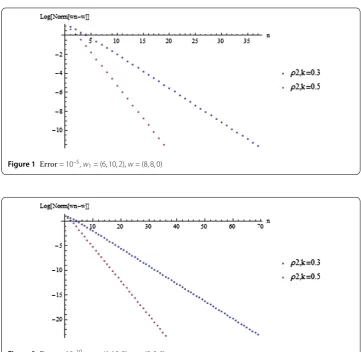
Figure 1 Error= 10–5,w
[image:12.595.116.478.75.427.2]1= (6, 10, 2),w= (8, 8, 0)
Figure 2 Error= 10–10,w
1= (6, 10, 2),w= (8, 8, 0)
In this algorithm, we takeρ2,k= 0.3, 0.5, respectively. Then we get some numerical
ex-periments which were run on a personal Dell computer with Intel(R)Core(TM)i5-4210U CPU 1.70 GHz and RAM 4.00 GB. And we wrote all the programs in Wolfram Mathemat-ica (version 9.0).
We take the initial valuew0= (6, 10, 2). Set the error to be 10–5, 10–10, respectively. Note
that we denote the number of iterations and the logarithm of the error by using the x-coordinate and the y-x-coordinate of the figures, respectively.
Acknowledgements
The authors would like to express their sincere thanks to the editors and reviewers for their noteworthy comments, suggestions, and ideas, which helped to improve this paper.
Funding
This research was supported by NSFC Grants No:11301379; No:11226125; No:11671167.
Availability of data and materials
All data generated or analysed during this study are included in this published article.
Competing interests
The authors declare that they have no competing interests.
Authors’ contributions
Publisher’s Note
Springer Nature remains neutral with regard to jurisdictional claims in published maps and institutional affiliations.
Received: 25 June 2019 Accepted: 7 October 2019
References
1. Moudafi, A.: Alternating CQ-algorithm for convex feasibility and split fixed-point problems. J. Nonlinear Convex Anal.
15(4), 809–818 (2013)
2. Moudafi, A.: A relaxed alternating CQ-algorithms for convex feasibility problems. Nonlinear Anal., Theory Methods Appl.79, 117–121 (2013)
3. Shi, L.Y., Chen, R.D., Wu, Y.J.: Strong convergence of iterative algorithms for split equality problem. J. Inequal. Appl.
2014, Article ID 478 (2014)
4. Dong, Q.L., He, S.N., Zhao, J.: Solving the split equality problem without prior knowledge of operator norms. Optimization64(9), 1887–1906 (2015)
5. Dong, Q.L., He, S.N.: Modified projection algorithms for solving the split equality problems. Sci. World J.2014, Article ID 328787 (2014)
6. Tian, D.L., Shi, L.Y., Chen, R.D.: Iterative algorithm for solving the multiple-sets split equality problem with split self-adaptive step size in Hilbert spaces. J. Inequal. Appl. (2016)
7. Bauschke, H.H., Combettes, P.L.: Convex Analysis and Monotone Operator Theory in Hilbert Spaces. Springer, London (2011)
8. Borwein, J.M., Li, G.Y., Tam Matthew, K.: Convergence rate analysis for averaged fixed point iterations in common fixed point problems. SIAM J. Optim.17(1), 1–33 (2017)
9. Bauschke, H.H., Borwein, J.M.: On projection algorithms for solving convex feasibility problems. SIAM Rev.38, 367–426 (1996)
10. Feng, M.L., Shi, L.Y., Chen, R.D.: Linear convergence of an iterative algorithm for solving the multiple-sets split equality problem. J. Nonlinear Funct. Anal. (2019)
11. Conway, J.B.: A Course in Functional Analysis, 2nd edn. GTM, vol. 96. Springer, Berlin (1989)