Clustering Algorithm of Quantum Self Organization Network

http://dx.doi.org/10.4236/ojapps.2015.56028

How to cite this paper: Li, Z.Y. and Li, P.C. (2015) Clustering Algorithm of Quantum Self-Organization Network. Open Jour-nal of Applied Sciences, 5, 270-278. http://dx.doi.org/10.4236/ojapps.2015.56028

Clustering Algorithm of Quantum

Self-Organization Network

Ziyang Li1*_{, Panchi Li}2

1_{School of Earth Science, Northeast Petroleum University, Daqing, China}

2_{School of Computer and Information Technology, Northeast Petroleum University, Daqing, China}

Email: *_{liziyangemail@126.com, lipanchi@vip.sina.com}

Received 22 May 2015; accepted 13 June 2015; published 16 June 2015

Copyright © 2015 by authors and Scientific Research Publishing Inc.

This work is licensed under the Creative Commons Attribution International License (CC BY). http://creativecommons.org/licenses/by/4.0/

Abstract

To enhance the clustering ability of self-organization network, this paper introduces a quantum inspired self-organization clustering algorithm. First, the clustering samples and the weight values in the competitive layer are mapped to the qubits on the Bloch sphere, and then, the winning node is obtained by computing the spherical distance between sample and weight value. Finally, the weight values of the winning nodes and its neighborhood are updated by rotating them to the sample on the Bloch sphere until the convergence. The clustering results of IRIS sample show that the proposed approach is obviously superior to the classical self-organization network and the K-mean clustering algorithm.

Keywords

Quantum Bits, Bloch Spherical Rotation, Self-Organization Network, Clustering Algorithm

1. Introduction

Since Kak [1] firstly proposed the concept of quantum inspired neural computation in 1995; quantum neural network (QNN) has attracted great attention by the international scholars during the past decade, and a large number of novel techniques have been studied for quantum computation and neural network. For example, Go-pathy et al.[2] proposed the model of quantum neural network with multilevel hidden neurons based on the su-perposition of quantum states in the quantum theory. Michail et al.[3] attempted to reconcile the linear reversi-ble structure of quantum evolution with nonlinear irreversireversi-ble dynamics of neural network. Michiharu et al.[4]

cal model of quantum neural network, building on Deutsch’s model of quantum computational network, which provides an approach for building scalable parallel computers. Fariel [6] proposed the neural network with the quantum gated nodes, and indicated that such quantum network may contain more advantageous features from the biological systems than the regular electronic devices. In our previous works [7], we proposed a quantum BP neural network model with learning algorithm based on the single-qubit rotation gates and two qubits con-trolled-rotation gates. Next, we proposed a neural network model with quantum gated nodes and a smart algo-rithm for it [8], which shows superior performance in comparison with a standard error back propagation net-work. Adenilton et al.[9] proposed a weightless model based on quantum circuit. It is not only quantum-in- spired but also actually a quantum NN. This model is based on Grover’s search algorithm, and it can both per-form quantum learning and simulate the classical models. At present, the fusion of quantum computation and neural computation is gradually becoming a new research direction.

In all of the above models, the fusion of quantum computing and supervised neural networks has been widely studied. However the fusion of quantum computing and unsupervised self-organizing neural network is rela-tively few. In the classical clustering algorithms, Cai et al.[10] proposed a new algorithm called K-Distributions for Clustering Categorical Data, and Huang [11] investigated clustering problem of large data sets with mixed numeric and categorical values. As it is known to all, unsupervised clustering is the only function of the self- organizing network. For self-organizing network, unsupervised clustering process, in essence, is the application process of the network. This is very different from BP network which must perform a supervised training process before application. Although we proposed quantum self-organizing networks with quantum inputs and quantum weights [12], this model applied the supervised mode to training, which severely reduces its generali-zation ability. In addition, although quantum computing effectively enhances the performance of the traditional self-organizing networks, the fusion research of quantum computation and neural computation is still far from mature. It is necessary to further research a new way of integration between them, in order to further improve the performance of neural computation. Hence, we proposed a quantum self-organization network based on Bloch spherical rotation (BQSON), and designed its clustering algorithm in detail. In our approach, both the samples and the weights are denoted by qubits described in Bloch sphere; the weights of the competition winning node and its neighbourhood nodes are adjusted by rotating these qubits to corresponding sample qubit about rotation axis. The experimental results of a benchmark of IRIS clustering show that our approach is superior to the traditional clustering methods such as common self-organizing networks, K-mean clustering, and the adjacent clustering.

2. The Spherical Description and Rotation of Qubits

2.1. The Spherical Description of Qubit

In the quantum computing, a qubit is a two-level quantum system which could be described in two-dimension complex Hilbert space. According to principle of superposition, a qubit can be defined as

i

cos 0 e sin 1

2 2

φ

θ θ

= +

ϕ (1)

where 0≤ ≤θ π, 0≤ ≤φ 2π.

Notation like is called the Dirac notation, and we will see it often in the following paragraphs, as it is the standard notation for states in quantum mechanics. Therefore, unlike the classical bit, which can only equal 0 or 1, the qubit resides in a vector space parameterized by the continuous variables θ and φ. The normalization condition means that the qubit’s state can be represented by a point on a sphere of unit radius, called the Bloch sphere. The Bloch sphere representation is useful as it provides a geometric picture of the qubit and of the transformations that can be applied to its state. This sphere can be embedded in a three-dimensional space of Cartesian coordinates (x=cos sinφ θ, y=sin sinφ θ, z=cosθ). Thus, the state ϕ can be written as

(

)

T

1 i

,

2 _{2 1}

z x y

z

 _{+ +} 

 

=

 + 

 

ϕ (2)

2.2. The Rotation of Qubit about an Aaxi on the Bloch Sphere

In this work, we adjust the weights of competition layer by rotating them around an axis towards the target qubit on the Bloch sphere. This rotation can simultaneously change two parameters θ and φ of a qubit and can au-tomatically achieve the best matching out of two adjustments, which can better simulate the quantum behaviour. To achieve this rotation, it is crucial to determine the rotation axis, as it can directly impact the convergence speed and efficiency of algorithm. To determine the rotation axis, we propose the following method.

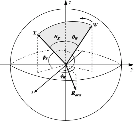
Let W = w wx, y,wz and X = xx,xy,xz denote two points on the Bloch sphere. The rotation axis for

rotating the qubit from W to X can be written as tensor product of W and X, and the relation of these three vec-tors is shown in Figure 2.

Let the Bloch coordinates of W and X be W = w w wx, y, z and X = x x xx, y, z. According to the

above method, the axis of rotating W to X can be written as

axis × =

×

W X

R

W X (3)

z

P

x

[image:3.595.140.543.207.579.2]

y

Figure 1. Qubit description on the Bloch sphere.

z

x

y

W X

[image:3.595.202.425.503.705.2]

From the principles of quantum computing, on the Bloch sphere a rotation through an angle δ about the axis directed along the unit vector n= n n nx, y, z is given by the matrix

( )

cos i sin

(

)

2 2

δ δ

δ = − ×

n

R I n σ (4)

where I denotes an unit matrix, σ = σ σ σx, y, z denotes the Pauli matrix as follows

0 1 0 i 1 0

, ,

1 0 i 0 0 1

x y z

−

     

=_{ } =_{ } =_{ }

−

     

σ σ σ (5)

Hence, on the Bloch sphere, a rotation through an angle δ about the axis Raxis that rotates the current

qu-bit W towards the target qubit X can be written as

( )

cos isin

(

)

2 2 axis

δ δ

δ = − ×

R

M I R σ (6)

and the rotation operation can be written as

( )

δ

= R

W M W (7)

2.3. The Measurement of Qubits

From the principles of quantum computing, the coordinates x, y, and z of a qubit on the Bloch sphere can be measured by the Pauli operators using the following equations.

0 1

1 0

x

x= = _ _

 

ϕ σ ϕ ϕ ϕ (8)

0 i

i 0

y

y= = _ −_

 

ϕ σ ϕ ϕ ϕ (9)

1 0

0 1

z

z= = _ _

−

 

ϕ σ ϕ ϕ ϕ (10)

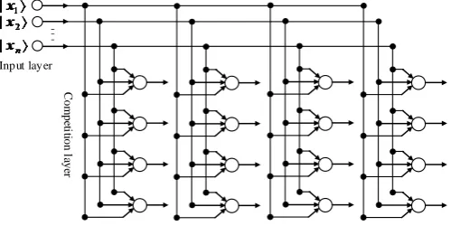
3. Quantum Self-Organization Neural Networks Model

We propose the quantum self-organization neural networks model based on the Bloch spherical rotation are shown in Figure 3, where both inputs and weight values are qubits described on the Bloch sphere.

Let X = x1 , x2 ,, xn T denote the inputs, and

T 1 , 2 , , j =  j j jn 

W w w  w denote the weight

values of the jth node in competition layer. By the projection measuring, the Bloch coordinates of xi and

ji

w can be written as xi = xix,xiy,xizT and

T

, ,

ji = wjix wjiy wjiz

w , respectively. From the spherical

geometry, the shortest distance between two points on a sphere is defined as the length of the minor arc on the big circle defined by these two points and the centre of Bloch sphere. As a result of the Bloch sphere radius equal

Input layer

C

om

pe

ti

tion l

aye

[image:4.595.189.439.581.706.2]

r

to 1, the spherical distance between xi and wji equal to the angle between them, and can be written as

(

)

(

)

arccos arccos

ij i ji ix jix iy jiy iz jiz

d = x w = x w +x w +x w (11)

Hence, the distance between X and Wj , namely, the output of the jth node in competition layer may be

given by

2 1 n j i ij

D =

∑

₌ d (12)

4. Quantum Self-Organization Neural Networks Algorithm

4.1. Quantum State Description of the Samples

First, all samples data are converted to [0, 1]. Let Xl =x l1,xl2,,xl nT,

(

l=1, 2,,L

)

denote the lthsample.

We adopt the following normalization method.

MIN

MAX MIN

l l

− =

−

X

X  (13)

where MAX and MIN respectively denote the maximum and the minimum of all samples.

Let sample after normalization be X_l = x_l1,x_l2,,x_{l n}_T, we use convert Xl to the phase of qubits by the

following equation

T T

1, 2, , π , π , , π1 2

l =θ θl l θl n = xl xl xl n

θ   (14)

T T

1, 2, , 2π , 2π , , 2π1 2

l =φ φl l  φl n = xl xl  xl n

ϕ (15)

At this point, Xl may be converted to qubits on the Bloch sphere, as shown in the following equation.

T

1 2 , ,

l = xl xl xl n 

X ，  (16)

where cos 0 ei sin 1

2 2

li

li li

li

x = θ + φ θ .

4.2. Competitive Learning Rules

Let Wj denote the weight value of the jth node in the competition layer, as follows

T

1 , 2 , ,

j = wj wj wjn 

W  (17)

For the lth sample X_l = x_l1 ，x_l2 ,, x_{l n }T, according to the Equations (11)-(12), the spherical dis-tance between Xl and Wj can be written as

(

)

2

1 arccos

n

lj i lix jix liy jiy liz jiz

D =

∑

₌ _ x w +x w +x w _ (18)

Suppose that the competition layer has C nodes, and that the node with a minimum distance is defined as the winning one. Hence, the winning node should satisfy the following equation

* 1min

lj lj

j C

D D

≤ ≤

= ₍₁₉₎

4.3. Network Clustering Algorithm

Step 1 Quantum state description of the sample. Convert the samples to qubit states by Equations (13)-(16). Measure the quantum samples by Equations (8)-(10) to obtain their Bloch coordinates.

Step 2 The weights of networks initialization. Initialize all the networks weights to randomly distribution of qubits on the Bloch sphere, as shown below.

T

1 , 2 , ,

j = wj wj wjn 

W  (20)

i

cos 0 e sin 1

2 2

ji

ji ji

ji

w = θ + φ θ (21)

where φji =2θji =2πrand, j=1, 2,,C, C denotes the number of competition nodes, and rand denote

the random number in (0, 1).

Step 3 The parameters of networks initialization. Include: the maximum iterative steps G, the initial value of learning rate β0, the finial value of learning rate βf, the initial value of neighbourhood radius r0, the finial

value of neighbourhood radius rf, the initial value of variance σ0, the finial value of variance σf . Set the

current iterative step t to 0.

Step 4 Compute the current learning rate, neighborhood radius, and variance by the following equations.

( )

0

(

0

)

( ) t G f t

β =β β β (22)

( )

(

)

( )

(

)

0 0 , 0.1

1 , 0.1

f

f

r r r t G t G

r t

r t G t G

 + − ≤

 = 

− >

 (23)

( )

0

(

0

)

( ) t G f t

σ =σ σ σ (24)

Step 5 Measure all quantum weights in competition layer by Equations (8)-(10) to obtain their Bloch coordi-nates. For the lth sample Xl

(

l=1, 2,,L

)

, compute the corresponding winning node

( )l

j∗

W by Equa-tions (18)-(19).

Step 6 For the lth sample Xl , in the competitive layer node array, select the neighborhood

(

( )

)

*

,

j r t

ψ

with the centre Wj( )∗l and the radius r t

( )

. For all nodes Wj in

(

( )

)

*

,

j r t

ψ , rotate each component

ji

w to the corresponding xli . The rotation angles are computed by the following equation

( )

( )

( )

_{( )}

(

)

2 , exp arccos 2 i

lj li ji

d j j

t t x w

t δ β σ ∗     = _− _     (25)

where d j j

( )

, ∗ denote the spherical distance between the jth node and the j*th node.

According to theorem, the rotation axis and rotation matrix of rotating wji to xli can be written as

,

, , , ,

, , , ,

jix jiy jiz lix liy liz ji li

jix jiy jiz lix liy liz

w w w x x x

w w w x x x

  × 

   

=

  × 

   

R ₍₂₆₎

( )

(

)

( )

( )

(

)

, cos i sin ,

2 2

i i

lj lj

i

ji li lj ji li

t t

t δ δ

δ = − ×

M I R σ (27)

Then, the rotation operation can be written as

( )

(

)

,

i

ji ji li lj li

w =M δ t x (28)

where j∈ψ

(

j r t*,

( )

)

, i=1, 2,,n, l=1, 2,,L.

Step 7 If t>G, save clustering results and stop, else set t = t + 1, and go back to Step 4.

5. Simulations

Clustering (NNC) in this section. In these experiments, we perform and evaluate the BQSON in Matlab (Version 7.1.0.246) on a Windows PC with 2.19 GHz CPU and 1.00 GB RAM. To enhance the impartiality of the com-parison results, our BQSON has the same structure and parameters as the CSON in this experiment. The IRIS data set contains 150 four dimensional samples. The sample is divided into three classes, and each class contains 50 samples, such as setosa (1 - 50), versicolor (51 - 100), virginica (101 - 150).

5.1. Parameter Settings

Both BQSON and CSON have 4 input nodes and 100 competition nodes arranged in square matrix. Other para-meters are set as follows: G=10000, β =0 0.8, β =f 0.1, r0 =5, rf =2, σ =0 5, σ =f 0.5.

If the clustering results do not change in 100 consecutive steps, we call algorithm reach convergence. For K-mean clustering, the K is set to 3, and if each of variations of class centers is less than 10

10− in two consecu-tive generations, the algorithm terminates. For NNC, the clustering threshold is set to λ=2.0. If the distance of the sample X from the center of the kth class is less than λ, the sample X is considered to belong to the kth class.

5.2. Clustering Result Contrasts

Considering the log likelihood function is more used in evaluation of the performance of the Bayesian classifi-cation network, and less used in clustering algorithm, therefore, we don’t use this index in our work. To facili-tate comparison, two relevant concepts are defined as follows:

Precision Ratio Let the correct number of samples in the kth class after clustering be NPR, and the total num-ber of samples in the kth class after clustering be NA. Precision Ratio is defined as follows

NPR

PR 100%

NA

= × (29)

Recall Ratio Let the correct number of samples in the kth class after clustering be NPR, and the total number of samples in the kth class before clustering be NB, Recall Ratio is defined as follows

NPR

RR 100%

NB

= × (30)

After 9797 iterative steps, the BQSON reaches convergence. All samples are divided into three classes, and each class contains 50 samples. The first class contains 50 “setosa” samples. The second class contains 48 “ver-sicolor” samples and 2 “virginica” samples. The third class contains 48 “virginica” samples and 2 “ver“ver-sicolor” samples. The Precision Ratio and Recall Ratio of three class samples reach 100%, 96%, 96%, respectively.

After 10,000 iterative steps, the CSON does not reach convergence, where the first class contains 50 “setosa” samples, and for the rest of the 100 samples, the model is powerless. In addition, we running until 30000 itera-tive steps, the CSON is still not convergence.

For K-mean clustering, after 11 iterative steps, convergence is reached. The first class contains 50 “setosa” samples, the second class contains 61 samples where 47 samples are correct, and the third class contains 39 samples where 36 samples are correct. The Precision Ratio of three class samples reach 100%, 77.05%, 92.31%, respectively, and the Recall Ratio of three class samples reach 100%, 94%, 72%, respectively.

For NNC, All samples are divided into three classes. The first class contains 50 “setosa” samples, the second class contains 62 samples where 50 samples are correct, and the third class contains 38 samples where all 38 samples are correct. The Precision Ratio of three class samplesreach 100%, 80.65%, 100%, respectively, and the Recall Ratio of three class samplesreach 100%, 100%, 76%, respectively.

5.3. Clustering Results Analysis

From the experimental results, it is clear that both Precision Ratio and Recall Ratio of BQSON are the highest in four algorithms. These results show that the BQSON is obviously superior not only to the CSON but to the K-mean and the NNC as well.

dis-tance measurement is generally taken the Euclidean disdis-tance, which this disdis-tance is calculated based on coordi-nates. In BQSON, however, the distance is obtained by calculating the Bloch spherical distance of each dimen-sion between input samples and competition nodes. Let yij

( )

t denote the jth output corresponding to the ith

input sample, where t denotes the current iterative step. Let

( )

1

( )

C

i j ij

y t =

∑

₌ y t C (31)

( )

( )

( )

2

1 C

i t j yij t y ti C

σ =

∑

₌_ − _ (32)

( )

1

( )

L i i

t t L

σ =

∑

₌σ (33)

where C denotes the number of nodes in competition layer, and L denotes the total number of samples. For the normalized samples, in CSON, the difference of each dimension between sample and weight dij

belongs to [0, 1]. In BQSON, the difference of each dimension ∈

[ ]

0,π belongs to

[ ]

0,π by applying the Bloch spherical distance. Hence, in order to make fair, we compared the average variance of BQSON after di-viding by _{π with that of CSON. The contrast results are shown in} 2 _{Figure 4.}

The Figure 4 shows that the average variance of BQSON is obviously greater than that of CSON, which suggests that the spherical distance have better distinguish ability than Euclidean distance for intensive samples. The “setosa” samples are relatively independent, which lead four algorithms to obtain the ideal clustering results. Both “versicolor” and “virginica” samples present overlapping intensive distribution, where the BQSON have also obtained the ideal clustering results. However, the clustering effect is not ideal for both K-mean and NNC based on the Euclidean distance, the CSON is completely unable to separate these two classes of samples.

Secondly, the BQSON adopted a new way of weight adjustment. In CSON, the vector differences between samples and weights are directly used to adjust the weighs, which is strongly influenced by learning rate, not easy to achieve fine adjustment. In BQSON, however, the weighs are adjusted by rotating them to a sample so as to approximate this sample. Due to the rotation is performed on the Bloch sphere, so, it may conduct a subtle adjustment of weights, which enhance the clustering ability of BQSON.

6. Conclusion

In this work, a quantum self-organization network clustering algorithm is proposed. In our approach, the weights of nodes in competition layer are updated by rotating qubits on the Bloch sphere. The comparative experiments of IRIS show that the clustering ability of proposed approach is significantly higher than the classic self-orga- nizing network. The Precision Ratio and Recall Ratio of BQSON increased by 7.5467% and 8.6667% more than those of K-mean and increased by 3.7833% and 5.3333% more than those of NNC. In addition, the BQSON is inefficient. It is also worth pointing out that, BQSON increases computing operations, such as the axis of rota-tion, rotation matrix and projection measurement, which lead to the increasing amount of calcularota-tion, prolonging running time, and reducing efficiency of clustering. However, the increase of these operations greatly improves

0 2000 4000 6000 8000 10000

0 0.05 0.1 0.15 0.15

iterative step

av

er

age v

ar

ianc

e

σ

qsom/π 2

σ

[image:8.595.193.429.538.703.2]

csom

the clustering ability of BQSON. In other words, BQSON is at the cost of computing efficiency for enhancing clustering ability, which is consistent with no free lunch theorem. Hence, how to enhance the computing effi-ciency of BQSON is the subject of further research.

Acknowledgements

This work was supported by the National Natural Science Foundation of China (Grant No. 61170132), Natural Science Foundation of Heilongjiang Province of China (Grant No. F2015021), Science Technology Research Project of Heilongjiang Educational Committee of China (Grant No. 12541059), and Youth Foundation of Northeast Petroleum University (Grant No. 2013NQ119).

References

[1] Kak, S. (1995) On Quantum Neural Computing. Information Science, 83, 143-160. http://dx.doi.org/10.1016/0020-0255(94)00095-S

[2] Gopathy, P. and Nicolaos, B.K. (1997) Quantum Neural Network (QNN’s): Inherently Fuzzy Feed forward Neural Network. IEEE Transactions on Neural Networks, 8, 679-693. http://dx.doi.org/10.1109/72.572106

[3] Michail, Z. and Colin, P.W. (1998) Quantum Neural Nets. International Journal of Theory Physics, 37, 651-684. http://dx.doi.org/10.1023/A:1026656110699

[4] Michiharu, M., Masaya, S. and Hiromi, M. (2007) Qubit Neuron According to Quantum Circuit for XOR Problem.

Applied Mathematics and Computation, 185, 1015-1025. http://dx.doi.org/10.1016/j.amc.2006.07.046

[5] Gupta, S. and Zia, R.K.P. (2001) Quantum Neural Network. Journal of Computer System Sciences, 63, 355-383. http://dx.doi.org/10.1006/jcss.2001.1769

[6] Fariel, S. (2007) Neural Network with Quantum Gated Nodes. Engineering Application of Artificial Intelligence, 20, 429-437. http://dx.doi.org/10.1016/j.engappai.2006.09.004

[7] Li, P.C. and Li, S.Y. (2008) Learning Algorithm and Application of Quantum BP Neural Network Based on Universal Quantum Gates. Journal of Systems Engineering and Electronics, 19, 167-174.

http://dx.doi.org/10.1016/S1004-4132(08)60063-8

[8] Li, P.C., Song, K.P. and Yang, E.L. (2010) Model and Algorithm of Neural Network with Quantum Gated Nodes.

Neural Network World, 11, 189-206.

[9] Adenilton, J., Wilson, R. and Teresa, B. (2012) Classical and Superposed Learning for Quantum Weightless Neural Network. Neurocomputing, 75, 52-60. http://dx.doi.org/10.1016/j.neucom.2011.03.055

[10] Cai, Z.H., Wang, D.H. and Jiang, L.X. (2007) K-Distributions: A New Algorithm for Clustering Categorical Data.

Proceedings of the 3rd International Conference on Intelligent Computing (ICIC’07), Qingdao, August 2007, 436-443.

http://dx.doi.org/10.1007/978-3-540-74205-0_48

[11] Huang, Z.X. (1997) Clustering Large Data Sets with Mixed Numeric and Categorical Values. Proceedings of the First

Pacific Asia Knowledge Discovery and Data Mining Conference, Singapore, World Scientific, 21-34.

[12] Li, P.C. and Li, S.Y. (2007) A Quantum Self-Organization Feature Mapping Networks and Clustering Algorithm.