AFRICAN BUFFALO OPTIMIZATION AND THE RANDOM IZED INSERTION ALGORITHM FOR THE ASYMMETRIC TRAVELLING SALESMANS PROBLEMS

ISSN: 1992-8645 www.jatit.org E-ISSN: 1817-3195

451

NEW ROBUST DESCRIPTOR FOR IMAGE MATCHING

1_{KABBAI LEILA,} 2_{ABDELLAOUI MEHREZ,} 3_{DOUIK ALI}

1,2,3

Research Laboratory of Automatic, Signal and Image Processing (LARATSI)

1,2

National Engineering School of Monastir- ENIM, University of Monastir-Tunisia

3

National Engineering School of Sousse- ENISo, University of Sousse-Tunisia

E-mail: [email protected], [email protected], [email protected]

ABSTRACT

Nowadays, object recognition based on feature extraction is widely used in image matching due to its robustness to different types of image transformations. This paper introduces a new approach for extracting invariant features from interest regions. This approach is inspired from the well known Scale Invariant Feature Transform (SIFT) interest points detector and aims to improve the computational efficiency of matching and object recognition while applying geometric and photometric transformations. To do so, we replace the Histogram of Gaussian (HoG) descriptor used in SIFT by other operators based on Local Binary Patterns (LBP), Gabor filter and Pyramid of Histograms of Oriented Gradients (PHOG). The novelty of this work is the construction of several descriptors based on Gabor, PHOG and LBP functions. Leading to seven new descriptors based on several combinations of the three proposed functions LBP, Gabor and PHOG at different layers. The performance of the proposed descriptors is evaluated using the recall vs. 1-precision curves and the average Areas Under Curve (AUC) metrics. Experiments show that the proposed descriptor called Histogram of LBP, Gabor and PHOG (HLGP) achieves more stable and robust results. Experimental evaluations demonstrate that HLGP outperforms the SIFT and the recent state-of-the-art descriptors.

Keywords: Scale Invariant Feature Transform (SIFT), Local Binary Patterns (LBP), Pyramid of Histograms of Oriented Gradients (PHOG), Gabor, image matching, local descriptor

1. INTRODUCTION

Image matching is an important task in computer vision applications, including object recognition [1], texture recognition [2], tracking [3], face detection [4]. Image matching can be defined as an estimation of the correspondences between two images based on local features. Local features were the subject of many researches in the recent few years. Applying local features in an image starts by detecting a set of points using an Interest Points (IPs) detector then describing these points using a local descriptor. In literature, different approaches have been proposed to detect IPs such as Moravec [5], Harris and Stephens [6], Harris-Lapace [7] and SIFT [8]. Mikolajczyk and Schmid [7] reported an experimental evaluation of several descriptors and found that the Scale Invariant Feature Transform (SIFT) algorithm obtained the best matching results when applying geometric and photometric transformations [9]. Various extensions of SIFT descriptor were developed in the recent years. Liu and al. [10] proposed a new approach called Simplified and Oriented Local Self-Similarities (SOLSS) which is a combination from the good properties of the SIFT and LSS. Also, Liu and al.

ISSN: 1992-8645 www.jatit.org E-ISSN: 1817-3195

452 extracting them in local regions around IPs. The experiments are applied on samples from the well known oxford database [16].

The manuscript is organized as follows: section 2 describes the SIFT, LBP, Gabor features and PHOG descriptor. Section 3 presents the proposed descriptors and their combinations. The experimental evaluation is carried out in section 4. Results and discussion are presented in section 5. Finally, a conclusion is given

2. FEATURE EXTRACTION

In this work, we developed a new method for image matching based on a combination of different descriptors. These descriptors are obtained from different methods such as SIFT algorithm, PHOG descriptor, LBP function and Gabor filter as features extracted for object recognition.

2.1 Scale Invariant Feature Transform (SIFT)

SIFT (Scale Invariant Feature Transform) algorithm proposed by Lowe in order to extract the most stable IPs of an image by using the Difference of Gaussian (DoG) and constructed a descriptor vector. This algorithm contains four main steps. - Scale-Space Extrema Detection: the DoG function is applied in scale space to extract the local extrema with invariance to scale and orientation. The extracted local extrema will be considered as IPs. - Interest Point Localization: to improve the robustness of the detected IPs, this step consists of discarding IPs with low contrast or with high response to DoG function and bad localization. - Orientation assignment: one or more orientations are assigned to every IP. This IP orientation constructs a 36 bins histogram of gradient.

- Interest point descriptor: Lowe proposes to generate a set of histograms over a window of 16-by-16 pixels around an IP. Typical IP descriptors use 16 orientations histograms aligned in a 4-by-4 grid. Every histogram has 8 orientations which leads to construct a 128 bins histogram considered as a feature vector.

2.2 Local Binary Patterns Feature (LBP)

The LBP operator is developed by Ojala and al. [17]. It is one of the best operators in describing texture information. It is robust against illumination changes and has good performances in terms of computational time. The LBP operator has been widely used in image retrieval [18], object

recognition [19] and leads to good results in face recognition [20]. The LBP algorithm operates by describing for each pixel a binary code computed after comparing a pixel gray level value to the values of its surrounding pixels in a 3-by-3 mask. In fact, as mentioned in equation 1, if the gray value of a neighbor is less than the central pixel, the result is assigned to be zero, otherwise to be one

.

∑

−

=

0

,

(

,

)

(

).

2

P

i

i c i R

P

x

y

s

g

g

LBP

(1)







≥

=

otherwise

x

if

x

s

0

0

1

)

(

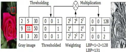
Where gc and gi represent respectively the gray

level value of the central and the neighborhood pixels. The parameters (P, R) are defined in table 1. The LBP value of a pixel is computed by multiplying the results with weights given by powers of two and summing the results as show in figure 1. The LBP value is between 0 and 255 and can be considered as a gray level value.

Figure 1 : The LBP Code Computation

2.3 Gabor Wavelets Feature

ISSN: 1992-8645 www.jatit.org E-ISSN: 1817-3195

453 )

, ( * ) ( ) ,

( _,

, x y z I x y

G_uv =ϕ_uv (2)

Gabor function φu,v (z) is obtained by multiplying

a Gaussian function and a complex exponential function as defined in equation 3.

 

 

 

 

− σ

= ϕ

σ − σ

−

2 2

2 2 , ,

2

, 2

2 2 ,

)

(z k e eik z e

z k v u v

u uv

v u

(3)

Where z=(x, y) are the spatial coordinates, u and v denote the orientation and scale respectively of the Gabor function. ||.|| defines the norm operator. ku,v is the wave vector illustrated in equation 4.

k

k

e

φ

=

,

where

8

;

/

u

f

k

k

=

φ

=

π

k max is the maximum frequency and fv is the

spacing factor. The parameter of Gabor filter presented in table 1. The Gabor feature is constructed by 40 bins vector G= [G1 G2… G40].

2.4 Pyramid of Histograms of Oriented Gradients Feature

Pyramid of Histograms of Oriented Gradient (PHOG) was firstly proposed by Bosch et al. [25]. It has been successfully applied to object classification in recent years. PHOG feature is used to describe the image at several repartition levels. This descriptor is inspired by the pyramid representation [26] and the Histogram of Orientation Gradients (HOG) [27]. PHOG descriptor is able to present a region in an image by its local shape and the spatial layout of the shape. The local shape is represented by a histogram of edge orientations within an image sub-region quantized into K bins and the spatial layout is represented by tiling the image into regions at multiple resolutions based on spatial pyramid. A HOG vector is calculated for each grid cell at each pyramid resolution level. The parameters of PHOG descriptor are illustrated in table l.

Table 1: Parameter Selection Of Many Functions

Figure 2 illustrates how the PHOG descriptor is obtained by the concatenation of all the HOG vectors at each pyramid resolution [28]. Therefore, the final PHOG descriptor of an image is a vector with size defined in equation 5.

bins K

L

L ₆₈₀

4 3

0

=

∑

=

Figure 2 : PHOG Descriptor At Each Level (0~2)

3. THE PROPOSED APPROACH

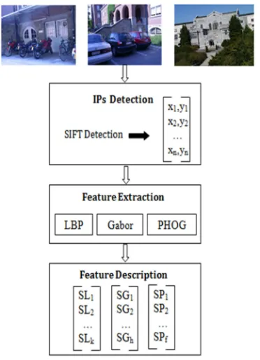
In this paper, we attempt to develop a novel descriptor based on histograms fusion. This technique was used successfully and showed high performances in different computer vision tasks such as image matching [29], texture classification [30] and object recognition [31]. The input of our algorithm is the same as the standard SIFT descriptor, with the same scale, space localization and orientation. Instead of computing the gradient features as the standard SIFT, we introduce different functions describing the local region. These functions are the LBP, Gabor and PHOG features. We used the LBP function which is based on texture features for describing interest regions. It has good performances in illumination changes and computational time. From this function, we obtained a new descriptor noted SIFT-LBP (SL) which is constructed by applying LBP function instead of gradient feature [32]. To build this descriptor, we extracted a patch of 16-by-16 pixels around the IPs. We divided the patch in 2-by-2 subregions. After that, we applied the LBPu2 function for each subregion to obtain a 59 bins

Function Description Value

LBP Circle of radius

Neighboring pixels

R=1 P=8

Gabor Scale _Orientation ν ∈ {0, … , 4}

u ∈ {0, … , 7}

PHOG

Number of pyramid levels Number of bins on the histogram

ISSN: 1992-8645 www.jatit.org E-ISSN: 1817-3195

454 histogram. We concatenated all histograms as vector of the size 59×4=236 bins. We proposed two other descriptors. The first one, called SG as SIFT-Gabor is based on SIFT-Gabor filter applied on IPs detected using SIFT detector. The second one is constructed when applying the pyramid HOG on IPs detected and is called SP as SIFT-PHOG. These two descriptors have respectively 40 and 680 bins as histogram size. Figure 3 illustrates the steps followed to build the different proposed descriptors.

Figure 3 : The Proposed Descriptors

In this step, we proposed two descriptors based on histogram fusion. First one is the fusion at histogram and the second is fusion at description.

3.1 Fusion At Histogram Detection Step

To improve the performance of the developed descriptors, we fused them at the histogram building step. The defined Histogram HLGP descriptor is obtained by histogram fusion of LBP, Gabor and PHOG functions as shown in figure 4. In fact, we fused the three histograms together to create 956 bins vector. In equation 6, we note that ki are bins obtained from LBP histograms, hi

represents bins obtained from Gabor filter histograms and fi are PHOG histogram bins.

}

{

[

]

}

{

[

]

The HLG descriptor (Eq. 7) is obtained by fusing LBP and Gabor histograms with a size of 276 bins.

Figure 4 : HLGP Descriptor

3.2 Fusion At Description Step

In this step, we build another approach to improve the matching by different combinations of SL, SG and SP descriptors concatenation. From these combinations, we have retained the two best performing descriptors. Descriptor of LBP and Gabor (DLG), illustrated in figure 5, which is a concatenation of SL and SG have a size of 276 bins and DLGP descriptor obtained by concatenating SL, SG and SP descriptors to form a vector of 956 bins. These descriptors are presented in equations 8 and 9.

[

]

[

]

Figure 5 : DLG Descriptor

ISSN: 1992-8645 www.jatit.org E-ISSN: 1817-3195

455 Table 2: Proposed Descriptors

4. PEXPERIMENTAL EVALUATION

The aim of these experiments is to evaluate the performance of our descriptor in an image matching task. We compared our proposed approach with other recent method, including SIFT-IGC [11], RATMIC [13], MROGH [14] and SIFT [8] descriptors which represents the reference of all methods developed for this task. This comparison is made on samples from Oxford dataset [16]. This dataset contains different groups of images with various geometric and photometric transformations such as blur variation for “Bikes” and “Trees” images, “Wall” images with different viewpoints and ambiguous textures. “Boat” set with zoom and rotation transformations. “Leuven” group of images with illumination variation. And “UBC” set with JPEG compression. Each transformation is applied with different levels on images from a group. However, each image is related to another one by the homography matrix of the applied transformation. The ground truth between the reference and other images are computed and given in the dataset. Figure 6 illustrates samples of pair of images from different categories.

( a ) ( b )

( c ) ( d )

( e ) ( f )

Figure 6 : Oxford dataset: (a) Bikes, (b) Leuven, (c) Wall, (d) UBC, (e) Trees, (f) Boat

4.1 Matching Strategy

The matching algorithm is based on the nearest neighborhood method. The similarity is measured using the Euclidean distance as shown in equation 10.

(

)

∑

=

−

= d

k

k k rj

ri rj

ri dist

1

2 )

,

(

Where ri and rj are respectively the descriptors vectors of images i and j, d is the size of the vector. We compute the nearest neighbor ratio R between dist1 and dist2 (Eq. 11) that represents respectively the similarity score between ri and rj1 and the

second similarity score between ri and rj2 [33].

threshold dist

dist

R = >

2

1

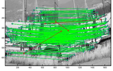
If R is less than the threshold, then the vectors are matched [34]. There are many mismatched points in the matching process. To remove the false matching, we used Random sample consensus (RANSAC) method. This method is robust to find out a mathematical model from a set of data and it has high performance in order to separate inliers (true) and outliers (false) matches [35]. This method was proposed by Fischeler and Bolles [36]. Figure 7 shows the matching between two image using SIFT descriptor and RANSAC method. Green lines in the figure correspond to inliers and red lines correspond to outliers.

Figure 7 : Image matching using RANSAC method

200 400 600 800 1000 1200 1400 1600 100

200 300 400 500 600

Methods Abbreviations Type

Fusion

Size (bins)

SIFT SIFT 128

SIFT- LBP SL 236

SIFT-Gabor SG 40

SIFT-PHOG SP 680

LBP-Gabor - PHOG

HLGP Histogram fusion

956

LBP-Gabor HLG Histogram fusion

276

LBPGabor -PHOG

DLGP Descriptor fusion

956

LBP-Gabor DLG Descriptor fusion

ISSN: 1992-8645 www.jatit.org E-ISSN: 1817-3195

456 4.2 Evaluation Criteria

To evaluate the performances of the developed descriptors, we define a set of evaluation criteria. These criteria are based on the inliers and outliers matching number. In fact, we employ recall versus 1-precision graphs by varying the distance threshold. The Recall is computed according to equation 12 and is equal to the number of correct matches divided by the number of correspondences which represents ground truth number of matching regions between the pair of images. Equation 13 defines the 1- precision rate which is based on the number of false and correct matches between two images.

number ences correspond

number matches correct

call =

Re (12)

number matches false number matches correct

number matches false ecision

+ =

−Pr

1 (13)

5. RESULTS AND DISCUSSION

In figures 8 to 12, we presented the experimental results applied on Oxford dataset. Experimental results demonstrate the superiority of the proposed method when compared to recent methods proposed for image matching under various image transformations.

5.1 Blur Variation

Image blur variation is a transformation made by adding a gaussian noise to the image with a standard deviation varying between 2 and 6. This transformation is applied on “Bikes” and “Trees” classes. To evaluate the performances of the proposed description under this transformation, we measure recall and precision criteria and plot the recall vs. 1-precision curve between images 1 and 6 for “Bikes” class (figure 8.a) and images 1 and 6 for “Trees” class (figure 8.b). We note that the HLGP descriptor leads to the best recall values when varying 1-precision. SG, SL and DLG descriptors have the worst results for this transformation.

(a)

(b)

Figure 8 : Recall vs. 1-Precision For Blur Variation (a) 1st and 6th From “Bikes”(b) 1st and 6th From

“Trees” Class

5.2 Illumination Variation

To evaluate the proposed descriptors under illumination variation, we used the “Leuven” class of images. The variation is created by changing the focus opening index of the camera. In figure 9, we note that HLGP and HLG gave the best results and are the only descriptors with results better than the standard SIFT.

Figure 9 : Recall vs. 1-Precision For Illumination Variation Applied On 1st And 6th From “Leuven” Class

0 0.1 0.2 0.3 0.4 0.5 0.6 0.7 0.8 0.9 1 0

0.1 0.2 0.3 0.4 0.5 0.6 0.7 0.8 0.9 1

Bikes

1-Precision

R

e

c

a

ll

SIFT SL SG SP HLGP HLG DLGP DLG

0 0.1 0.2 0.3 0.4 0.5 0.6 0.7 0.8 0.9 1

0 0.1 0.2 0.3 0.4 0.5 0.6 0.7 0.8 0.9 1

Trees

1-Precision

R

e

c

a

ll

SIFT SL SG SP HLGP HLG DLGP DLG

0 0.1 0.2 0.3 0.4 0.5 0.6 0.7 0.8 0.9 1

0 0.1 0.2 0.3 0.4 0.5 0.6 0.7 0.8 0.9 1

Leuven

1-Precision

R

e

c

a

ll SIFT

ISSN: 1992-8645 www.jatit.org E-ISSN: 1817-3195

457 5.3 JPEG Compression

In this step, we use a set of JPEG compression images. Figure 10 depicts the results between image1 and image 4 for “UBC” class using the recall vs. 1-precision curve. We observe in figure 10 that HLGP, HLG and DLGP descriptors give better results than the SIFT descriptor. SL, SG, SP descriptors obtain slightly lower results than SIFT descriptor.

Figure 10 : Recall vs. 1-Precision For JPEG Compression Applied On 1st And 4th From “UBC”

Class

5.4 View Point Changes

View point changes are applied on “Wall” class. This transformation is done by changing the acquisition viewpoint.

Figure 11 : Recall vs. 1-Precision For View Point Changes Applied On 1st And 4th From “Wall” Class

In figure 11, we evaluate the proposed descriptor between images 1 and 4. We note that SP, HLG, DLGP and HLGP descriptor have better results than SIFT. DLGP reach recall value exceeding 95%.

5.5 Zoom and rotation transformation

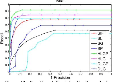
Zoom and rotation transformation is applied in same time on Boat images. Figure 12 shows that HLGP, HLG, DLGP and SP descriptors are significantly better than SIFT when computing recall vs. 1-precision curves.

Figure 12 : Recall vs. 1-Precision For Zoom And Rotation Transformation Applied On 1st And 2nd From

“Boat” Class

5.6 Area Under Curve

Recall vs. 1-precision curve shows the performances of the proposed descriptors but not precisely. To be more precise we compute the Area Under Curve value (AUC) for every curve and each class. In table 3, we illustrate the AUC value for each descriptor when applied to different classes from the Oxford dataset. We note that the HLGP descriptor have the best mean AUC value exceeding 0.7. This descriptor is selected to be compared to recent developed method in image matching that used the same dataset.

Table 3: Average Area Under Curve For Recall vs. 1-Precision Curves

0 0.1 0.2 0.3 0.4 0.5 0.6 0.7 0.8 0.9 1

0 0.1 0.2 0.3 0.4 0.5 0.6 0.7 0.8 0.9 1

UBC

1-Precision

R

e

c

a

ll SIFT

SL SG SP HLGP HLG DLGP DLG

0 0.1 0.2 0.3 0.4 0.5 0.6 0.7 0.8 0.9 1

0 0.1 0.2 0.3 0.4 0.5 0.6 0.7 0.8 0.9 1

Wall

1-Precision

R

e

c

a

ll SIFT

SL SG SP HLGP HLG DLGP DLG

0 0.1 0.2 0.3 0.4 0.5 0.6 0.7 0.8 0.9 1

0 0.1 0.2 0.3 0.4 0.5 0.6 0.7 0.8 0.9 1

Boat

1-Precision

R

e

c

a

ll SIFT

SL SG SP HLGP HLG DLGP DLG

Dataset SIFT SL SG SP HLGP HLG DLGP DLG

Bikes 0,501 0,465 0,427 0,650 0,724 0,654 0,493 0,463

Leuven 0,644 0,585 0,415 0,601 0,734 0,727 0,658 0,605

UBC 0,927 0,804 0,887 0,922 0,972 0,963 0,966 0,870

Wall 0,681 0,238 0,228 0,693 0,893 0,800 0,866 0,370

Boat 0,750 0,442 0,546 0,830 0,890 0,829 0,776 0,620

Trees 0,087 0,030 0,023 0,128 0,216 0,184 0,147 0,038

ISSN: 1992-8645 www.jatit.org E-ISSN: 1817-3195

458 5.7 Comparison To Recent Methods

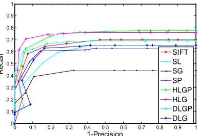
The HLGP descriptor is compared to the recent descriptors proposed in image matching such as: SIFT-IGC [11], RATMIC [13], MROGH [14]. In figure 13 and 14, we can see that our descriptor achieves best results compared to SIFT-IGC for different transformations such as blur variation (Fig. 13. (a) and (b)), Illumination variation (Fig. 13. (c)), JPEG compression (Fig. 14. (a)) and view point changes (Fig. 14. (b)). The mean value of AUC measure for these transformations reaches 0,708. Whereas the SIFT-IGC AUC

value for the

same transformation is equal to 0,626.

Also in figure 14, we observe that our descriptor obtained best results compared to RATMIC and MROGH descriptors for JPEG compression (Fig.14. (a)), view point changes (Fig.14. (b)) and for zoom and rotation transformation (Fig.14. (c)). The mean value of AUC measure for these transformations reaches 0,9183. This value outperforms MROGH descriptor with an AUC value equal to 0,9179. The RATMIC descriptor presents the worst results with a value around 0,825.

(a)

(b)

(c)

Figure 13 : Illustration Of HLGP Descriptor Performance Compared To SIFT and SIFT-IGC In Terms

Of Recall vs. 1-Precision Curves. (a) And (b) Blur Variation, (c) Illumination Variation

(a)

(b)

0 0.1 0.2 0.3 0.4 0.5 0.6 0.7 0.8 0.9 1 0

0.1 0.2 0.3 0.4 0.5 0.6 0.7 0.8 0.9 1

Bikes

1-Precision

R

e

c

a

ll

SIFT HLGP SIFT-IGC

0 0.1 0.2 0.3 0.4 0.5 0.6 0.7 0.8 0.9 1 0

0.1 0.2 0.3 0.4 0.5 0.6 0.7 0.8 0.9 1

Trees

1-Precision

R

e

c

a

ll

SIFT HLGP SIFT-IGC

0 0.1 0.2 0.3 0.4 0.5 0.6 0.7 0.8 0.9 1

0 0.1 0.2 0.3 0.4 0.5 0.6 0.7 0.8 0.9 1

Leuven

1-Precision

R

e

c

a

ll

SIFT HLGP SIFT-IGC

0 0.1 0.2 0.3 0.4 0.5 0.6 0.7 0.8 0.9 1

0 0.1 0.2 0.3 0.4 0.5 0.6 0.7 0.8 0.9 1

UBC

1-Precision

R

e

c

a

ll

SIFT HLGP SIFT-IGC RATMIC MROGH

0 0.1 0.2 0.3 0.4 0.5 0.6 0.7 0.8 0.9 1

0 0.1 0.2 0.3 0.4 0.5 0.6 0.7 0.8 0.9 1

W all

1-Precision

R

e

c

a

ll

ISSN: 1992-8645 www.jatit.org E-ISSN: 1817-3195

459

(c)

Figure 14 : Illustration of HLGP Descriptor Performance Compared To SIFT, SIFT-IGC, RATMIC

And MROGH Descriptors In Terms Of Recall vs. 1-Precision Curves. (a) JPEG Compression And (b) View Point Changes, (c) Zoom And Rotation Transformation

6. CONCLUSION

In this paper, we propose a new method for describing interest regions called HLGP descriptor. This descriptor is based on shape and texture feature extraction methods respectively inspired from PHOG, LBP, Gabor functions. To do so, we replace the histogram of Gaussian descriptor applied in SIFT by the proposed HLGP descriptor. The novelty of this work is the construction of a vector based on histogram fusion of features extracted from LBP, Gabor and PHOG functions. Experimental evaluations show that the proposed HLGP descriptor applied on image matching leads to the best results compared to the standard SIFT descriptor and new descriptors from the state-of-art. The Empirical results are based on the computation of the recall vs. 1-precision curves and their related AUC values measured for different photometric and geometric transformations from the Oxford dataset.

REFRENCES:

[1] Lowe, D.G.: “Distinctive image features from scale-invariant keypoints”, International Journal of Computer Vision, 2004, 60, (2), pp. 91–110. [2] Lazebnik, S., Schmid, C., Ponce, J.: “A sparse

texture representation using local affine regions”, IEEE Transactions on Pattern Analysis and Machine Intelligence, 2005, 27, (8), pp.1265-1278.

[3] Abdellaoui, M., Kabbai. L, Douik A.: “New matching method for human body tracking”,

Proc. Int. Conf. Multi-Conference on systems, Signals and Devices, Barcelona, Febrary2014, pp.1-5.

[4] Hirdesh, K., Padmavati: “Face Recognition using SIFT by varying Distance Calculation Matching Method”, International Journal of Computer Applications, 2012, 47, (3), pp.20-26 [5] Moravec, H P.: “Towards automatic visual

obstacle avoidance”, International Joint Conference on Artificial Intelligence, 1977, (2), pp. 584-584.

[6] Harris C., Stephens M.: “A combined corner and edge detector”, Alvey Vision Conference, 1988, pp.147-151.

[7] Mikolajczyk, K., Schmid, C.: “A performance evaluation of local descriptors”, IEEE Transactions on Pattern Analysis and Machine Intelligence, 2005, 27, (10), pp. 1615-1630. [8] Lowe, D.G.: “Object recognition from local

scale-invariant features”, International Conference on Computer Vision, Kerkyra, 1999, 2, pp.1150-1157.

[9] Kaur, J., Kaur, N.: “Modified Sift Algorithm for Appearance Based Recognition of American Sign Language”, International Journal of Computer Science Engineering & Technolo, 2012, 2(5), pp.1197-1202.

[10] Liu, J., Zeng, G.: “Description of interest regions with oriented local self-similarity”, Optics Communications, 2012, 285, (10-11), pp. 2549-2557.

[11] Liu, J., Zeng, G.: “Description Improved Global Context descriptor for describing interest regions”, Journal of Shanghai Jiaotong University (Science), 2012, 17, (2), pp 147-152. [12] Su, D., Wu, J., Cui, Z., Cui, et al.: “CGCI-SIFT:

A More Efficient and Compact Representation of Local Descriptor”, Measurement Science Review, 2013, 13, (3), pp.132-141.

[13] Huang, Z., Kang, W., Wu, Q., et al.: “A new descriptor resistant to affine transformation and monotonic intensity change”, Computer Vision and Image Understanding, 2014, 120, pp.117-125.

[14] Bin, F., Wu, F., Hu, Z.: “Rotationally Invariant Descriptors Using Intensity Order Pooling”, IEEE Transactions on Pattern Analysis and Machine Intelligence, 2012, 34, (10), pp 2031-2045.

[15] Heikkilä, M., Pietikäinen, M., Schmid C.: “Description of Interest Regions with Local Binary Patterns, pattern recognition”', Pattern Recognition, 2006, 42, 3, pp. 425-436.

0 0.1 0.2 0.3 0.4 0.5 0.6 0.7 0.8 0.9 1

0 0.1 0.2 0.3 0.4 0.5 0.6 0.7 0.8 0.9 1

Boat

1-Precision

R

e

c

a

ll

ISSN: 1992-8645 www.jatit.org E-ISSN: 1817-3195

460 [16] Mikolajczyk, K., Tuytelaars, T., et al.: “Affine

Covariant Features”,

http://www.robots.ox.ac.uk/~vgg/research/affin e/, 2010.

[17] Ojala, T., Pietikainen, M., Maenpaa, T.: “Multiresolution gray scale and rotation invariant texture analysis with local binary patterns”, IEEE Transactions on Pattern Analysis and Machine Intelligence, 2002, 24, (7), pp. 971-987.

[18] Yu, J., Qin, Z., Wan, T., et al.: “Feature integration analysis of bag-of-features model for image retrieval”, Neurocomputing, 2013, 120, pp. 355-364.

[19] Satpathy, A., Jiang, X., Eng, H.L.: “LBP-based edge-texture features for object recognition”, IEEE Transactions on Image Processing, 2014, 23, (5), pp. 1953-1964.

[20] Abdur, R., Najmul, H., Tanzillah, W., et al.: “Face Recognition using Local Binary Patterns (LBP)”, Global Journal of Computer Science and Technology Graphics & Vision, 2013, 13,(4) ,pp. 1-7.

[21] Gabor, D.: “Theory of communication”, Journal of the Institution of Electrical Engineers-Part III: Radio and Communication Engineering, 1946, 93, (26), pp. 429-457.

[22] Zhang, S., Zhao, X., Lei, B.: “Facial Expression Recognition Using Sparse Representation”, WSEAS transactions on systems, 2012, 11, (8), pp. 440-452.

[23] Xuejuan, K., Panpan, Y., Junfeng J.: “Defect Detection on Printed Fabrics Via Gabor Filter and Regular Band”, Journal of Fiber Bioengineering and Informatics, 2015, 8, (1), pp. 195-206.

[24] Yanuar, W., Romi, S.W., Vincent, S. : “Color and Texture Feature Extraction Using Gabor Filter - Local Binary Patterns for Image Segmentation with Fuzzy C-Means”, Journal of Intelligent Systems, 2015, 1, (1), pp. 15-21. [25] Bosch, A., Zisserman, A., Munoz, X.:

“Representing shape with a spatial pyramid kernel”. Proc. Int. Conf. on image and video retrieval, 2007, pp .401-408.

[26] Lazebnik, S., Schmid, C., Ponce, J.: “Beyond bags of features: Spatial pyramid matching for recognizing natural scene categories”, Computer Vision and Pattern Recognition, 2006, 2, pp. 2169-2178.

[27] N. Dalal and B Triggs, “Histogram of oriented gradients for human detection”, IEEE Computer Society Conference on Computer Vision and

Pattern Recognition , San Diego, CA, USA, 2005, pp. 886-893.

[28] Huang, H.M., Liu, H.S., Liu, G.P.: “Face Recognition Using Pyramid Histogram of Oriented Gradients and SVM”, Advances in information Sciences and Service Sciences, 2012, 4, (18), pp.1-8.

[29] Mikolajczyk, K., Schmid, C.: “A performance evaluation of local descriptors”, IEEE Transactions on Pattern Analysis and Machine Intelligence, 2005, 27, (10), pp. 1615-1630. [30] Zhang, J., Marszalek, M., Lazebnik, S., Schmid,

C.: “Local features and kernels for classification of texture and object categories: A comprehensive study”, International Journal of Computer Vision, 2007, 73, (2), pp. 213-238. [31] Li, J., Allinson, N. M.: “A comprehensive

review of current local features for computer vision”, Neurocomputing, 2008, 71, issue (10-12), pp 1771–1787.

[32] Kabbai, L., Azaza, A., Abdellaoui, M., Douik, A.: “Image Matching Based on LBP and SIFT Descriptor”, IEEE International Multi-Conference on Systems, Signals and Devices, Mahdia, March 2015.

[33] Kabbai, L., Abdellaoui, M., Douik, A.: “Hybrid classifier using SIFT descriptor”. Proc. Int. conf. on Control, Decision and Information Technologies, Hammamet, May 2013, pp. 388-392.

[34] Strachan, E.: “The application of range imaging for improved local feature representations”, PhD thesis, University of Glasgow, 2013. [35] Liang, J., Liao, Z., Yang, S., et al.: “Image

matching based on orientation–magnitude histograms and global consistency”, Pattern Recognition, 2012, 45, (10), pp. 3825-3833. [36] Fischler, M.A., Bolles, R.C.: “Random sample