The use of frequency domain parameters to predict structural fatigue

(1)

University of Warwick institutional repository: http://go.warwick.ac.uk/wrap

A Thesis Submitted for the Degree of PhD at the University of Warwick

http://go.warwick.ac.uk/wrap/34794

This thesis is made available online and is protected by original copyright. Please scroll down to view the document itself.

(2)

The use of frequency domain parameters

to predict structural fatigue

by

N. W. M. Bishop

A Dissertation submitted for the Degree of

Doctor of Philosophy

Department of Engineering

University of Warwick

December 1988

(3)

Summary

The work in this thesis outlines the use of power spectral density data for estimating the Fatigue Damage of structures or components subjected to random loading. Since rainflow cycle counting has been accepted as the best way of estimating the fatigue dam-age caused by random loadings, an obvious target was a method of obtaining the rainflow range distribution from the PSD. Such a solution is derived in this thesis. It forms the major part of the work presented and appears in chapter 5. The rest of the thesis deals with the following topics;

Chapter 3 first presents some empirical solutions developed by other authors for the prediction of rainflow ranges from PSD's. An empirical solution developed by Dirlik in 1985 is then used to investigate the effect that stresses contained within a given fre-quency range have on fatigue damage when there are other frequencies present in the PSD plot. This can be thought of as 'fatigue damage potential'. Interactions between stresses in different frequency intervals are investigated and it is shown that the fatigue damage potential of one frequency interval is dependent not only on the magnitude of that interval but on the magnitudes of other frequency intervals present. This 'Interac-tion' effect within the PSD plot, is of specific interest because it can be used to determine the change of fatigue damage for any given structure or component when parts of the sig-nal or PSD plot are altered.

Chapter 4 is concerned with methods of regenerating a signal from a PSD in the form of a set of peaks and troughs. Work by Kowalewsld in 1963 is introduced which gives a solution for the joint distribution of peaks and troughs. This distribution can be used to generate a continuous set of adjacent peaks and troughs, of any length, using Monte-Carlo techniques. Approximations in this result are discussed, in comparison with the (distribution of times between) zero crossings problem. An improvement to this joint distribution of peak and troughs is given which uses an empirical solution for the distri-bution of 'ordinary ranges' (ranges between adjacent peaks and troughs).

Chapter 5 forms the major part of the original work presented in this thesis and out-lines a theoretical solution for the prediction of rainflow ranges using statistics computed directly from the power spectral density plot. The rainflow range mechanism is broken down into a set of logical criteria which can be analyzed using Markov process theory. The dependence between extremes in this instance is modelled using the prediction of the joint distribution of peaks and troughs proposed by Kowalewsld, and shown in chapter 4.

Chapter 6 deals with the fatigue damage assessment and stress history determination of components when only limited samples of the service data are available. An investiga-tion is carried out into the relative merits of time and frequency domain techniques. In particular, the effect of finite sample length was investigated with particular reference to the variance of fatigue predictions using both a rainflow count on a limited time sample and a rainflow count produced directly from a PSD of the same time sample. The fre-quency domain approach is shown to be at least as accurate as the direct time domain approach.

(4)

Table of contents

Summary _(i)

Table of contents _(ii)

List of tables and figures _(v)

List of abbreviations and symbols _(xi)

Acknowledgements (xvi)

Declaration (xvii)

1.0 Introduction 1

1.1 References 7

2.0 Theoretical tools for the statistical and fatigue damage analysis of ran- 9 dom signals

2.1 Basic fatigue theory 9

2.2 Cycle counting methods 10

2.3 Probability theory and random variables 13

2.3.1 General assumptions 13

2.3.2 One random variable 14

2.3.3 Two random variables 15

2.4 Power spectra 16

2.5 Random variables which follow a Gaussian (normal) distribution 19 2.6 The statistical analysis of signals which are stationary, ergodic, Gaus- 20

sian and random using the joint distributions of x, ±-_{dt T}_{x ' -}

d r

d x

and

2.7 The narrow band solution for calculating the fatigue damage from fre- 22 quency domain statistics

2.8 The distribution of times between zero crossings 24

2.9 References 27

3.0 An investigation of the fatigue damage potential of individual fre- 35 quency components within any power spectral density plot using an

empirical solution for the prediction of 'ordinary' and `rainflow' ranges

3.1 Introduction 35

ix 3.2 Previous solutions to the rainflow range program 36 3.3 A general solution for fatigue damage including the wide band case 38

3.4 Computer programs used for investigation 39

3.4.1 Stage 1. Computation of fatigue damage using narrow band, rainfiow 40 range and ordinary range solutions

3.4.2 Stage 2. Fatigue damage potential of individual frequency components 42 3.4.3 Stage 3. Interactions between discrete frequency components within 43

the PSD.

3.5 Conclusions 44

(5)

4.0 Signal regeneration using Markov matrices - an improved solution to 66 Kowalewski's joint peak-trough probability density function.

4.1 Introduction 66

4.2 Kowalewsld's solution for the joint distribution of peaks and troughs. 68

4.2.1 The distribution of maxima 69

4.2.2 The number of points of inflection per second 71 4.2.3 Kowalewski's joint distribution of peaks and troughs 72 4.3 An improvement to Kowalewski's solution for the joint distribution of 76

peaks and troughs.

4.4 Generating time signals in the form of a set of peaks and troughs 77 4.5 Cycle counting from a series of peaks and troughs 78

4.6 Results and conclusions 80

4.7 References 83

5.0 A theoretical solution for the prediction of `rainflow' ranges from 102 power spectral density data

5.1 Introduction 102

5.2 Historical background to the theory of rainflow range predictions from 103 power spectral density plots.

5.3 A new theoretical solution for the prediction of rainflow ranges. 105

5.4 Markov chains. 107

5.5 Modelling the problem 108

5.6 Outline of computational solution 112

5.6.1 Generation and acquisition of 'real data' 112

5.6.2 Rainflow range count on original signal 112

5.6.3 Power spectral density computation 112

5.6.4 A rainflow count from a set of peaks and troughs generated from 113 Kowalewski's joint probability density function

5.6.5 A rainflow range density function produced using the new theoretical 113 solution

5.7 Results and discussion. 113

5.8 References 116

6.0 The use of frequency domain techniques to characterise the amplitude 133 content of short lengths of signal.

6.2 Generating realistic data 135

6.3 Data acquisition 135

6.4 Data qualification 136

6.5 Cycle counting from time signals, with particular reference to short 138 lengths of signal

(6)

6.7 Computational procedure for estimating the fatigue damage from both 141 time and frequency domain information

6.8 The variance of fatigue predictions from limited sample sizes using 142 both time and frequency domain methods

6.9 Conclusions 144

6.10 References 145

7.0 The dynamic fatigue damage analysis of fixed offshore platforms, with 179 some examination of structures subjected to wind loading.

7.2 Recap of other Authors work and relevant theory 181

7.2.1 Sea Environment Characterisation 181

7.2.2 Wave Model 183

7.2.3 Member Force Calculation 186

7.2.4 Structural Behaviour 188

7.2.5 Spectral Analysis 190

7.2.6 Fatigue Damage Model 192

7.3 Present Methods of Analysing Wave Loadings 192

7.3.1 Deterministic 193

7.3.2 Transient 195

7.3.3 Spectral 197

7.3.4 Deterministic/Spectral 200

7.3.5 Transient/Spectral 201

7.3.6 Probabilistic 202

7.4 One approach to the analysis of wind loading 202

7.5 Analysis used for this investigation 206

7.5.1 ASAS#G 207

7.5.2 ASAS#WAVE 208

7.5.3 ASAS#RESPONSE 210

7.5.4 ASAS#FATJACK 210

7.5.5 N2 211

7.5.6 N12 212

7.6 Results 212

7.7 Conclusions 216

7.8 References 221

8.0 Conclusions and suggestions for future research 276

(7)

List of tables and figures

Figure 1.1. A typical stress response PSD plot from a location in a component or 8 structure which exhibits dynamic response.

Figure 2.1. A typical stress-life (S-N) diagram. 30 Figure 2.2. The time response which results from the mixture of a low and high 31 frequency.

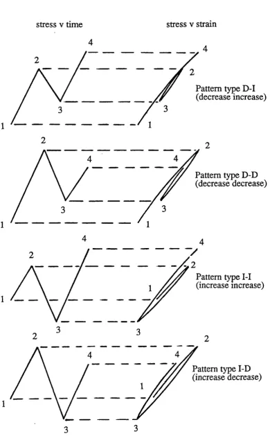
Figure 2.3. The four different types of pattern which are considered in the Pat- 32 tern Classification Procedure.

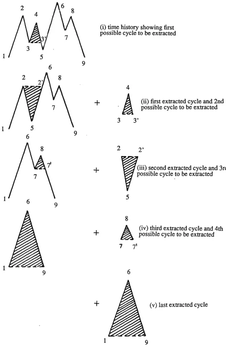
Figure 2.4. An example of the use of the Pattern Classification Procedure for 33 rainflow cycle counting a short length of time signal.

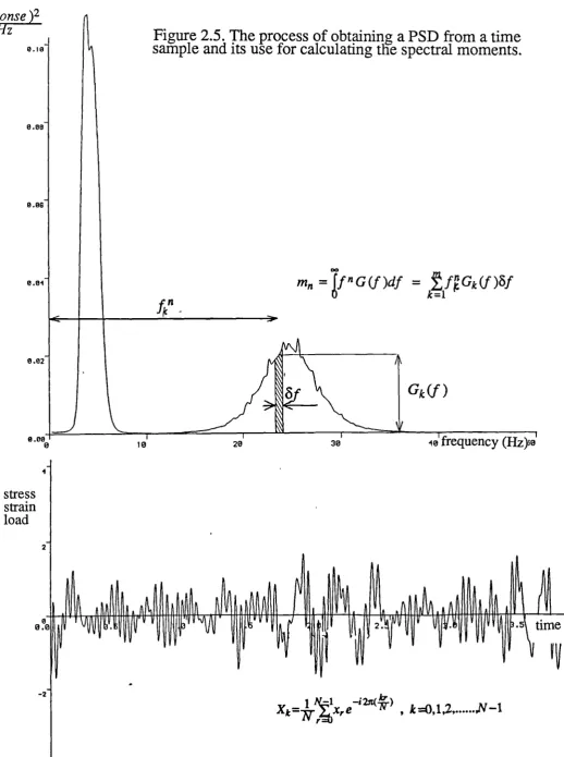
Figure 2.5. The process of obtaining a PSD from a time sample and its use for 34 calculating the spectral moments.

Table 3.1. Fatigue damage calculations using the narrow band, ordinary range 48 and rainflow range methods for 11 sea states which are typical of the

environ-mental conditions experienced in the north sea.

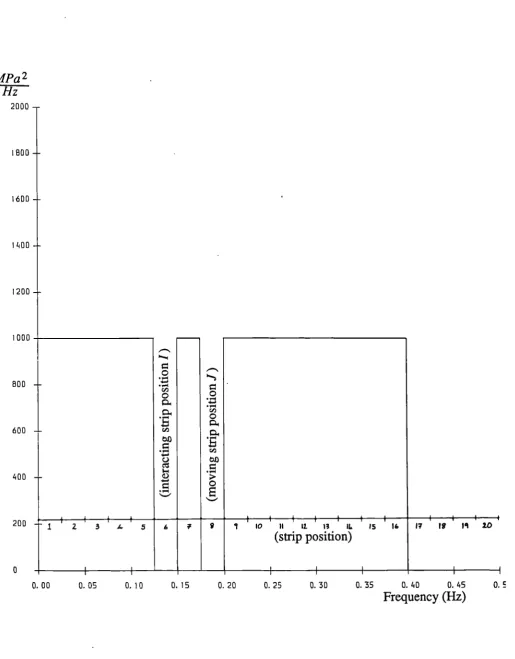
Table 3.2. A numerical example of the application of equation 3.13, showing 49 'primary' interactions between frequency components within a rectangular PSD

as shown if figure 3.17.

Table 3.3. The numerical results for primary interactions at moving strip 11 50 showing that the sum of the effects of the interacting strips is approximately

equal to the fatigue damage potential of strip 11.

Table 3.4. Damage results for different values of the following; the number of 51 frequency points used (Ai), the number of points used in the range probability

function (L) and the range probability function integration limit (iN times the rms).

Figure 3.1. Basic outline of the three stages of programs used for the investiga- 52 tion.

Figure 3.2(a)-3.12(a). Sea state 1-11 53-58

Figure 3.2(b)-3.12(b). Narrow band, ordinary and rainflow range probability 53-58 density functions computed from sea state 1-11 using equations 2.57, 3.4, 3.5.

Figure 3.13. The fatigue damage caused by one isolated strip which does not 59 take into account the effect of interactions between frequencies.

Figure 3.14. The fatigue damage potential of particular frequencies within sea 59 state 1 calculated with the narrow band, ordinary range and rainflow range

methods.

Figure 3.15(a). A rectangular PSD with a thin strip removed from a location 60 which is stepped along the frequency axis and called a 'moving strip'.

Figure 3.15(b). The effect on fatigue damage of removing one small strip from 60 the PSD.

Figure 3.16(a). A rectangular PSD which also has an additional strip present at 61 some remote point.

Figure 3.16(b). The effect on fatigue damage of removing one small strip from 61 the PSD is now seen to be affected by the additional strip present at some

(8)

Figure 3.17. The method used to assess the effect of primary interactions. 62 Figure 3.18. The effect of an interacting strip on the fatigue damage potential of 63 a particular moving strip computed using rainflow ranges.

Figure 3.19. The effect of an interacting strip on the fatigue damage potential of 64 a particular moving strip computed using ordinary ranges.

Figure 3.20. The effect of an interacting strip on the fatigue damage potential of 65 a particular moving strip computed using the narrow band assumption.

Figure 4.1(a). Kowalewski's peak-trough joint probability density function 85 (equation 4.38), for sea state 1.

Figure 4.1(b). A contour plot of Kowalewsld's peak-trough joint probability 85 density function (equation 4.38), for sea state 1.

Figure 4.2(a). Kowalewski's peak-range joint probability density function 86 (equation 4.42), for sea state 1.

Figure 4.2(b). A contour plot of Kowalewski's peak-range joint probability den- 86 sity function (equation 4.42), for sea state 1.

Figure 4.3(a). The authors modified peak-range joint probability density func- 87 tion (equation 4.44), for sea state 1.

Figure 4.3(b). A contour plot of the authors peak-range joint probability density 87 function (equation 4.44), for sea state 1.

Figure 4.4. The use of a peak-range joint probability density function for gen- 88 erating a time history of peaks and troughs.

Figure 4.5. The first 251 points in a peak-trough series generated from 89 Kowalewski's peak-range joint probability density function, for sea state 1.

Figure 4.6. The narrow band, ordinary and rainflow range probability density 90 functions computed from sea state 1 using equations 2.57, 3.4, 3.5.

Figure 4.7. The peak distributions computed from time series of Kowalewski's 90 and the modified peak-range joint distributions compared with the theoretical

prediction (equation 2.53), for sea state 1.

Figure 4.8. Dirlik's ordinary range solution compared with the ordinary range 91 predictions computed from both the Kowalewski and the modified joint

distribu-tions (equadistribu-tions 4.42 and 4.44), for sea state 1.

Figure 4.9. Dirlik's rainflow range solution compared with the rainflow range 91 predictions computed from both the Kowalewski and the modified joint

Figure 4.10. Kowalewski's peak-range joint probability density function (equa- 92 tion 4.42), for sea state 7.

(9)

Figure 4.14. Dirlik's ordinary range solution compared with the ordinary range 94 predictions computed from both the Kowalewski and the modified joint

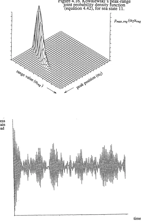
Figure 4.16. Kowalewslci's peak-range joint probability density function (equa- 95 tion 4.42), for sea state 11.

prediction (equation 2.53), for sea state 11.

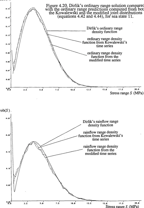
Figure 4.20. Dirlik's ordinary range solution compared with the ordinary range 97 predictions computed from both the Kowalewsld and the modified joint

Figure 4.22. The bth moment of the ordinary range density functions computed 98 from both the Kowalewsld and the modified joint distributions after being

nor-malised by the bth moment of Dirlik's ordinary range density function, for sea state 1.

Figure 4.23. The bth moment of the rainflow range density functions computed 98 from both the Kowalewski and the modified joint distributions after being

nor-malised by the bth moment of Dirlik's rainflow range density function, for sea

state 1.

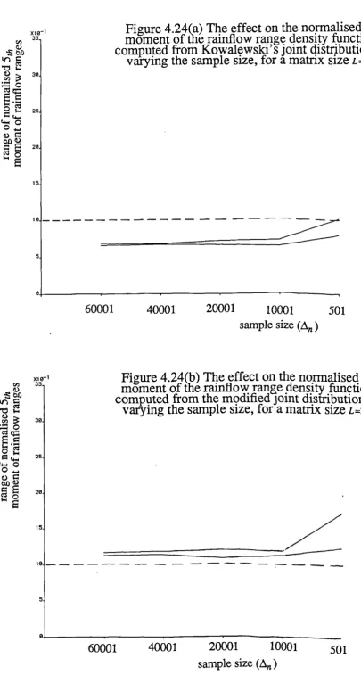
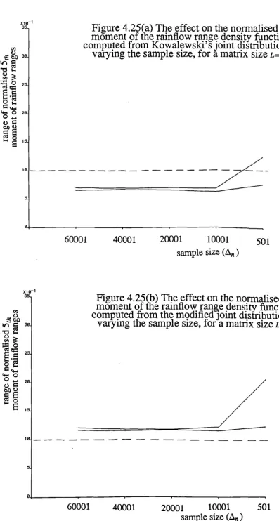
Figure 4.24(a)-4.26(a) The effect on the normalised 5th moment of the rainflow 99-101 range density function computed from Kowalewski's joint distribution of

vary-ing the sample size, for a matrix size L=33, 65 and 101.

Figure 4.24(b)-4.26(b) The effect on the normalised 5th moment of the rainflow 99-101 range density function computed from the modified joint distribution of varying

the sample size, for a matrix size L=33, 65 and 101.

Figure 5.1. The concept of upper and lower bounds on damage compared with 118 that computed using rainflow ranges.

Figure 5.2. Rychlik's definition of a rainflow range cycle. 119 Figure 5.3. Discrete form of the authors definition of a rainflow range cycle. 120 Figure 5.4(a). Kowalewski's expression for the dependence between adjacent 121 extremes.

Figure 5.4(b). Kowalewski's expression for the dependence between adjacent 122 extremes after both the peak-trough and the trough-peak parts have been

nor-malised to 1.

(10)

Figure 5.5(b). The trough-peak part of l‘pwalewsld's expression (equation 2) for 123 a 16 by 16 element matrix.

Figure 5.6. The Markov process model used to characterise the steps of figure 2 124 which are necessary to fully define a rainflow range cycle for a particular peak.

Figure 5.7(a). Transition matrix representing peak-trough (1 step) movements 125 for the particular configuration of ip=10 and kp =3.

Figure 5.7(b). Transition matrix representing trough-peak (1 step) movements 125 for the particular configuration of ip=10 and kp =3.

Figure 5.8(a). Transition matrix representing peak-trough-peak (2 step) move- 126 ments for the particular configuration of ip=10 and kp =3.

Figure 5.8(b). Condensed transition matrix representing peak-trough-peak (2 126 step) movements for the particular configuration of ip =10 and kp=3.

Figure 5.8(c). Condensed transition matrix after it has been squared enough 126 times to ensure state 4 is empty (2 steps, where n is the number of times the

matrix is squared).

Figure 5.9(a-c). A comparison of the rainflow range distributions obtained (data 127-129 set 2 with 16, 32 and 63 element matrices) using equation 1 (new theoretical

solution) with a distribution obtained from a peak-trough count of, (1) the origi-nal sigorigi-nal, and (2) a sigorigi-nal regenerated from a Kowalewski peak-trough matrix.

Figures 5.9(d-f). A comparison of the rainflow range distributions obtained (data 130-132 sets 1, 3 and 5 and 32 element matrix) using equation 1 (new theoretical

solu-tion) with a distribution obtained from a peak-trough count of, (1) the original signal, and (2) a signal regenerated from a Kowalewski peak-trough matrix.

Tables 6.1-6.5. qualification tests carried out on data sets 1-5 147-156 Table 6.6. Results showing the effect of quantisation on accuracy. 157 Figure 6.1. The output characteristics of the Briiel and Kjaer random signal gen- 158 erator

Figure 6.2. The output of one of the low pass filters set to 250 Hz. 159 Figure 6.3(a-e). Power Spectral Density plot computed from data sets 1-5 160-164 Figure 6.4. The effect of quantisation of the signal on the range distributions. 165 Figure 6.5. A study of the percentage error caused by the moment integration 166 elemental strip width (Dx), for various values of (b), the slope of the S-N curve,

(X) the range value and (A) and (D), the vertical and horizontal axis

intersec-tions with a straight line representing the range distribution.

Figure 6.6. The eighth possible combinations of the signal tails shown along 167 with the most justifiable method of joining the ends together.

Figure 6.7(a). Comparison of ordinary ranges computed directly from full data 168 set with ordinary ranges computed from PSD of full data set using equation 3.4.

Figure 6.7(b). Comparison of rainflow ranges computed directly from full data 168 set with rainflow ranges computed from PSD of full data set using equation 3.5.

(11)

Figure 6.13(b). Narrow band frequency domain prediction of fatigue (using 172 equation 2.58), normalised by rainflow range prediction of time signal ... plotted

against sample size

Figure 6.14(a). rms computed from PSD of time sample, normalised by popula- 173 tion rms ... plotted against sample size

Figure 6.14(b). rms computed from time sample, normalised by population rms 173 Figure 6.15(a) Number of peaks per second calculated from PSD of time sample 174 (using equation 2.8), normalised by population number of peaks per second ...

plotted against sample size

Figure 6.15(b) Number of peaks per second calculated from time sample, nor- 174 malised by population number of peaks per second ... plotted against sample

size

Figure 6.16(a). Ordinary range frequency domain prediction of fatigue (using 175 equation 3.4), normalised by ordinary range prediction from PSD of full time

signal ... plotted against sample size

Figure 6.16(b). Ordinary range time domain prediction of fatigue, directly from 175 time signal, normalised by ordinary range prediction on full time signal ...

plot-ted against sample size

Figure 6.17(a). Rainflow range frequency domain prediction of fatigue (using 176 equation 3.5), normalised by rainflow range prediction from PSD of full time

signal ... plotted against sample size

Figure 6.17(b). Rainflow range time domain prediction of fatigue, directly from 176 time signal, normalised by rainflow range prediction on full time signal ...

plot-ted against sample size

Figure 6.18(a). Ordinary range prediction of fatigue from Kowalewski's regen- 177 erated signal, normalised by ordinary range prediction on full time signal ...

Figure 6.18(b). Ordinary range prediction of fatigue using the authors regen- 177 erated signal, normalised by ordinary range prediction on full time signal ...

Figure 6.19(a). Rainflow range prediction of fatigue from Kowalewski's regen- 178 erated signal, normalised by rainflow range prediction on full time signal ...

Figure 6.19(b). Rainflow range prediction of fatigue using the authors regen- 178 erated signal, normalised by rainflow range prediction on full time signal ...

Table 7.1. Statistical properties and damage expectations computed from 225 Wirsching' s data

Table 7.2(i). base wave cases used in ASAS#WAVE 225

Table 7.2(ii). Full ASAS results 226

Table 7.3. N12 results for fatigue damage caused by sea states 1 to 11 228 Table 7.4. N12 results for fatigue damage potential estimation. 231 Table 7.5. The variation of DN with A,,, and B„, 232

(12)

Figure 7.1. The variation of force with depth for different wave periods 234 Figure 7.2(a). Velocity, acceleration and force curves along the wave profile 235 Figure 7.2(b). Results for one vertical member from an ASAS#WAVE run 236 Figure 7.3. The relative effects of the drag and inertia terms on the wave force 237 Figure 7.4. Frequency response plot for a one degree of freedom system 238

Figure 7.5. The interaction effects within any PSD plot 239

Figures 7.6(a-c). Velocity, acceleration and force spectra for sea states 1,6 and 240-242 11

Figure 7.6(d). Velocity, acceleration and force spectra for sea state 6, with van- 243 ous member diameters

Figure 7.7. An example of the Deterministic/spectral method 244

Figure 7.8. The effects of varying the parameters A,,, and B,,, on fatigue damage 245

Figure 7.9. A flow chart of the programs used for analysis 246

Figure 7.10. Plots of structures A and B using ASAS#ASDIS 247

Figure 7.11. The first eight mode shapes for structure B 248

Figure 7.12(a). The sin fitting process with 12, 6 and 4 phase increments for an 249 inertia dominated wave

Figure 7.12(b). The sin fitting process for a drag dominated wave 250 Figure 7.12(c). The sin fitting process for a drag dominated wave in the splash 250 zone

Figure 7.13(a). Height against force. Conservative linearisation 251 Figure 7.13(b). Height against force. Unconservative linearisation 251

Figure 7.14. The process of obtaining the transfer function 252

Figure 7.15. The variation of fundamental frequency with added mass 253 Figure 7.16. The variation of fatigue life with critical damping 254 Figures 7.17(a-k). Results for sea states 1-11 with transfer function H3 255-265 Figures 7.18(a-k). Fatigue damage potential for sea states 1-11 255-265 Figure 7.19. Different methods of estimating the fatigue damage potential of 266 any response plot

Figure 7.20. The variation of fatigue life with a wave angle of 0 degrees 267 representing waves square on to the side

Figure 7.21. The variation of fatigue life or damage with elevation of water 268 level at 0.0, representing a water level at a horizontal bracing level

Figure 7.22. The maximum response of a structure comprising of a 3 by 3 array 269 of piles for varying wavelength

Figure 7.23. The maximum response of a structure comprising of a 3 by 3 array 270 of piles for varying wavelength and waveangle

(13)

List of abbreviations and symbols

symbols and notation used throughout this in the text.

c(b) = coefficient in Wirsching's

correc-tion factor (3.2).

C = sub determinant of A (4.29) C = factor in equation 4.9. C = sub matrix of P (5.7).

C = factor used in equation 7.118.

C = damping factor (7.28).

C (f ) = characteristic function (2.10).

C ( f ,g) = joint characteristic function (2.20).

CI ,C2 = coefficients in Dirlik's expression for ordinary ranges (3.4).

of Cinan) = characteristic function of max-ima (4.31).

Cinfux(n) = characteristic function of points of inflection (4.32).

• = factor used in equation 4.44. • = inertia coefficient (7.13).

CD = drag coefficient (7.14).

C i,C2 = factors used in equation 7.16. Cc = critical damping factor (7.28)

• = multiplying weighting constant (7.60).

d = factor used in equation 4.9. d = depth to mean water level. dN = increment of H-N curve.

D = intersection of S-N curve line with horizontal axis.

D diameter of incremental section of member (7.15).

D = sub determinant of A (4.29).

D = fatigue damage (7.49).

D i ,D 2

p

3 = coefficients in Dirlik's expres-sion for rainflow ranges (3.5).

dh=Dh = stress range interval width. This section lists the more common

thesis along with a reference to the first use

a = factor used in equation 4.7.

a = water particle acceleration (7.6(b)). • = covariance of x ix; (2.33).

a (b) = coefficient in Wirsching's

conec-don factor (3.2).

A = matrix in n dimensional normal dis-tribution (2.31).

A = intersection of S-N curve line with vertical axis.

A = coefficient in equation 3.9. A = sub matrix of P (5.7).

A = factor used in equation 7.118.

A = area of incremental section member (7.15).

A = factor in equation 7.25.

• = cofactor of au (2.33).

1,

•

A2 = factors used in program N2. Ai = factor used in equation 4.44. A 1 ,A2 = factors used in equation 7.38.

aN = normal acceleration (7.55).

ar = tangential acceleration (7.55). A (t) = factor given by equation 7.58(f). A„, = factor used in equation 7.88. b = slope of S-N curve.

b = factor in equation 4.7. B = factor used in equation 4.7.

B = sub matrix of P (5.7).

B = factor used in equation 7.118. Bi = factor used in equation 4.44. B = factor used in equation 4.44.

b 2 = slope of H-N curve (7.44).

B (t) = factor given by equation 7.58(g).

• = factor used in equation 7.88.

(14)

Di = factor used in equation 4.44. • = factor used in equation 4.44. Di = total damage in id, sea state.

DN = normalised damage (7.100). erf (x) = error function

ejwi = (coswt — jsinwt) (7.35).

E[] = expected or mean value (2.5).

E [P] = expected number of peaks per unit

time (2.50).

E [P1] = expected number of points of inflection per unit time (2.51).

E [0] = expected number of zeros per unit time (2.49).

E [a] = expected number of level cross-ings per unit time (2.48).

E[D]ris = fatigue damage based on the narrow band assumption (2.56).

E[D]oR = fatigue damage calculated using ordinary ranges (3.8).

E[D]RR = fatigue damage calculated using rainflow ranges (3.6).

f = frequency in Hertz.

f = natural frequency (3.9).

je,"k = long term transition probability. = expected frequency of observations (6.1).

ID = frequency of wave spectrum peak

(7.2(b)).

f (t) = fluctuating force (7.87). fR = _{B (7.88).}_fl,

F = load or force (7.29). = Fast Fourier Transform.

F 1 ,F 2 = factors used in program N2.

Fi = observed frequency of observations (6.1).

Fl = inertia component of force (7.12).

FD = drag component of force (7.12). FT = total force (7.12).

FTAPP = approximation to FT (7.16). F = maximum load or force (7.29).

F(r) load or force as function of time (7.36)

F(t) factor given by equation 7.58(e).

F„(z ,t) = force at depth z on member n at time t.

= static force (7.87).

FDN denormalising factor (7.100). FT' = force on one pile (7.120). Fm = force on N piles (7.120). g = gravity.

g (a) = probability density function of peaks (2.53).

G (r) = factor given by equation 7.70).

Gk(I) = G (f) = single sided PSD in units of Hertz (2.27).

h = stress range (see section 3.2). H = wave height.

H, = significant wave height (3.9) H (jw) = transfer function (7.37).

H„, = maximum wave height in 100 years (7.44).

ip = level of point 1 (see section 5.3).

JN = integration limit for range functions. k = coefficient from S-N curve.

kp = level of point 2 (see section 5.3). k = wave number (7.5).

K = factor in equation 4.7.

K = stiffness (7.20).

K = factor used in equation 7.86. = factor given by equation 7.58(d).

= factor used in equation 7.68. L = wave length.

L = matrix size (see section 4.4).

(15)

XL. = length scale (7.91).

M(s) = moment generating function (2.8). PZ(S ,t) = joint moment generating

func-tion (2.18).

m„ = nth moment of _{G (f)}(2.28(a)).

M = mass (7.20).

MG = factor used in equation 7.97).

n = number of cycles at a particular stress range.

It, = number of sinusoidal components used to fit wave profile (7.54).

N = allowable number of cycles at a

par-ticular stress range.

N,,, = number of waves in 100 years

(7.44).

Ni = number of waves in the id, sea state

(7.52).

NG = total number of wind speed

fluctua-tions (7.94).

p (x) = probability density function (2.3).

p (x ,y) = joint probability density function

(2.14).

POR = probability density function of

ordinary ranges (3.4).

PRR = probability density function of

rainflow ranges (3.5).

P (x 11X 2tX 3, rYpt ) = n dimensional

proba-bility density function.

p (s) = probability density function of stress ranges (2.55).

Pamp(aa) = probability density function of amplitudes (4.37).

Nin,max(alia2) = joint probability density function of peaks and troughs (4.38).

p„,,a,„p(a„„ '3(0 = joint probability density -function of means and amplitudes (4.39).

Pnwitg(a.,anig) = joint probability density

function of means and ranges (4.40).

Pmax,amp(a2,400 = joint probability density

function of peaks and amplitudes (4.41).

Pn la x,rng(a2,armg) = joint probability density

function of peaks and ranges (4.42).

11,1.(1 ,j) = joint probability density

func-tion calculated from elemental probabili-ties.

p (S,,) = probability density function of normalised stress range (7.96).

P SD = Power Spectral Density.

P = transition matrix (5.4),

P (x,y) = joint probability distribution function (2.12).

P (x) = probability distribution function (2.2).

P hi' 2,1 ' 4 = sub matrices of? (5.6).

P (R ,Q) = empirical distribution for the heights of sea waves (7.4).

p (H) = Rayleigh distribution (7.51).

Q = coefficient used in Dirlik's expres-sion for rainflow ranges (3.5).

Q1,Q2 = factors used in program N2 Q i = sub matrix of P (5.6).

Q = normalised wave period (7.4). Q(t) = total force on structure (7.77).

r = wave amplitude (7.4). rms = root mean square value.

Rzy (T) = cross correlation function (2.22).

Rxx CO = R (r) = auto correlation function

(2.23).

R = coefficient in Dirlik's expression for

rainflow ranges (3.5).

R 31 ,R 32,R 34 = sub matrices of _{P (5.6).}

R = normalised wave height (7.4).

RFF = auto correlation function of wave

force on one pile (7.69).

RA = auto correlation of wave force on N piles (7.78).

S = stress range (2.55).

S = stress range (3.6).

(16)

SRR (h) = rainflow range probability

den-sity function (5.1).

Szy(c)) = cross spectral density function (2.25(a)).

S (f) = Pierson Moskowitz sea state spectrum (7.2(a)).

SRR(f) = response PSD (7.40).

SFF(f) = force PSD (7.41).

SDD(f ) = displacement PSD (7.42).

S (f) = stress response PSD (7.43).

S(H)=a ill +a2H2

Sd = dynamic response including a dynamic amplification function (7.50).

Sgg (f. = PSD representing the sum of a

number of random processes (7.60). Sfig) = PSD of generalised forces

(7.64).

Szaz,(f ) = PSD of generalised modal coor-dinates (7.65).

s(f) = PSD after transformation back into original coordinates (7.66).

SFF(f) = PSD of loading component

(7.75).

S (f) = PSD of water particle velocities (7.72(a)).

S (f) = PSD of wind speed fluctuations (7.88).

Saa(f) = PSD of water particle accelera-tions (7.72(b)).

Sik(f) = PSD of wave forces on N piles (7.79).

SFF Or = PSD of loading component (7.75).

SFF (f ) = PSD of loading component

(7 .7 5).

-SFF(f) = PSD of loading component (7.75).

= normalised stress range (7.95).

T = wave period (7.4).

TD = dominant wave period.

Tz = zero crossing period (7.3).

Tmin = lowest natural period of structure (7.59).

Tffp(f) = transfer function between PSD of force on one pile and the PSD of force on N piles (7.82).

T(f)= transfer function (7.83).

u = stress range level at y(t) (see section 5.3).

U = water particle velocity (7.6(a)). Limy = rms of velocity fluctuations (7.19).

V(r) = fluctuating wind velocity (7.87). 17 = mean wind velocity (7.87).

vz = hourly-mean wind speed (7.91). V3p = sub matrices of P (5.12).

= nth moment of S(w) (2.28(b)).

WI = circular frequency of oscillation of a

one degree of freedom system (7.22). x (t)= variable as function of time.

x(k) = discrete samples taken of X (t).

= mean value of x(k). 3Ch = FF1 of x(k) (2.26).

dm x m x =

dtm

xy, = coefficient used in Dirlik's expres-sions (3.4,3.5).

Xm = coefficient used in Dirlik's

expres-sions (3.4,3.5).

x0= maximum displacement (7.31).

xt, = horizontal space coordinate for the nth pile in an N pile array measured in the direction of wave travel (7.79).

xi = horizontal distance from some refer-ence point (7.120).

z = water depth at calculation point (7.6(a)).

Z = transformed variable given by

equa-tion 7.26.

Z = normalised variable (3.7).

lim > 0 (5.10).

(17)

AD = damage at a particular wave height (7.48).

At = increment of time.

An = number of segment lengths (see sec-tion 4.4).

n = '41-- (7.33). WI

0 = phase shift (7.32).

na = iim P a (5.10).

= correct estimate (6.2). tP. = approximate estimate (6.2).

9 = angle of attack of waves onto side of structure (7.82).

lir1 = condition 1 of rainflow range test.

Y2 = condition 2 of rainflow range test. Y3 = condition 3 of rainflow range test.

Y(v) = 1+0.25v2 (7.4).

cc = Philips constant (7.2(a)). a = factor used in equation 7.56.

a„ = nth moment (2.6).

a = variable used for displacement (2.34). al = trough value.

a2 = peak value. a. = mean value. R„ = amplitude value.

J3 = variable used for velocity (2.34). f3 = a constant used in equation 7.2(a). 13 = factor used in equation 7.56. f3a = 17--c-(I32-131) (4.24).

f3„, = * (132+13 1) (4.24).

X2 = chi squared value (6.1).

5 = wave orbit (7.11).

-Sx = elemental probability box size (see section 4.4).

= time between samples (see section 6.1(a)).

5, = error in estimation (6.2).

c = A-171g.

ri = distance of sea surface elevation from mean water level (7.2(a).

gi = critical damping in the ith mode (7.57).

y = irregularity factor (2.52). yf = factor used in equation 7.16.

X(b ,e) = Wirsching's correction factor (3.2).

g = variable used for derivative of acceleration.

v = factor used in equation 7.4. c.o = circular frequency.

4) = coefficient (3.9).

4) = variable used for coordinate transfor-mation (7.26).

'WO = nth moment of Rx, (t) at . 0 (2.59).

nv, = nth moment of R.,, (r) (2.59).

y = factor used in equation 7.68.

p = mass density of water (7.15).

al = variance of x(k) (2.7).

a. = standard deviation.

a = rms (for zero mean valued variable = ax).

cq = variance of wind speed fluctuations (7.89).

as = rms of stress ranges (7.95).

t = time separation.

T = coefficient in Dirlik's expression for

ordinary ranges (3.4)

T = factor used in equation 7.4.

= damping factor (3.9).

C = variable used for acceleration (4.5). Ca = , (Cz-Ci) (4.25).

(18)

Acknowledgements

First of all I would like to thank SERC, the University of Warwick and the Depart-ment of Engineering for their financial support during the period of this research.

My supervisor was Dr Frank Shenatt and I would like to express my deep apprecia-tion for his encouragement, guidance and advice over the past three and a half years.

(19)

Declaration

This dissertation is submitted in support of an application for the Degree of Doctor of Philosophy in Engineering Science, from the University of Warwick.

No part of the work contained in the thesis has been submitted for other Degrees or Diplomas from this University or any other Institution.

The work contained in this thesis is original and my own unless otherwise stated in the text.

I declare that this declaration is true in every respect.

(20)

1. Introduction

The work in this thesis outlines the use of power spectral density data for estimating the Fatigue Damage of structures or components subjected to random loading. Fatigue has been defined as (ref.1.1);

The process of progressive localized permanent structural change occurring in a material subjected to conditions which produce fluctuating

stresses and strains at some point or points and which may culminate in cracks or complete fracture after a sufficient number of fluctuations.

Most basic research into material fatigue has been concerned with metals. In these, the fundamental process of crack formation is now known to result from an intensification of slip lines, or dislocations within crystals, caused by repeated loading. These cracks may propagate until total collapse of the component or structure occurs. Despite the fact that a thorough understanding of the physics underlying these processes is now available (refs.1.2,1.3), most engineering design is based on an empirical approach.

The particular empirical approach used will depend on the type of component being designed. For instance, a nuclear plant pressure vessel will have been classified as failed after the appearance of a crack. However, in an offshore platform tubular joint it may be acceptable for the structure to remain in service with cracks of much greater size than the minimum which can be detected, perhaps of 5mm or more. This leads to the idea of cracks appearing and growing in size without impeding the integrity of the structure or component.

Various analysis techniques have emerged to deal with such differing design requirements. These include;

(21)

2

(b) The fracture mechanics approach. Crack propagation is assumed to depend on a fracture mechanics parameter, usually the range of crack tip stress AK. Life is then calculated by assuming an initial crack length and finding how many cycles are needed to make this crack grow to an unacceptable size.

(c) The local stress-strain or critical location approach. The strain history of some critical location is estimated from the loading history, including plasticity effects. Life is then estimated from test data taken under strain controlled con-ditions. Prediction of life to crack initiation is the objective.

The nominal stress approach was used for the work described in this thesis when-ever a particular choice of methods was necessary, therefore parts of the thesis which deal specifically with aspects of fatigue analysis have direct relevance to this method. It was chosen because methods such as the ones described above, either have no relevant influence on the focus of the present study, or are unsuitable for dealing with the loading problems investigated. Loading problems arise because there is a need to define a stress (or strain) 'cycle' of loading. This is required whenever the loading conditions are more complex than constant amplitude. The main purpose of the work in this thesis is to investigate such loading conditions using modern ideas on cycle counting.

W.5 hler (ref.1.4) first pointed out many very important aspects of fatigue behaviour, the most important being that fatigue depends more on the range of stress than the max-imum stress. He also suggested that the fatigue life of specimens reduces when the amplitudes of repeated loading increases, introducing the concept of stress versus life (S-N) diagrams. Because of the apparent simplicity of this relationship it has formed the basis of much present day fatigue design. The diagram is traditionally produced using results from tests carried out at constant load amplitudes.

(22)

3

-unaffected by the presence of a different stress range. Having ignored the possible consequences of the above assumptions there is still a problem to be solved when the loading is irregular, because of the way different frequencies and magnitudes of the sig-nal are mixed together. This makes it difficult to extract cycles of stress on which to apply Miner's rule. This is typical of random vibrations in a car body shell or where dynamic responses are present in structures such as offshore oil platforms.

The appearance of `rainflow cycle counting' (ref. 1.6) has provided an answer to the problem of what constitutes a 'cycle'. It has now generally been accepted that rainflow cycle ranges give the best agreement with actual fatigue lives (ref.1.7). Furthermore, when the service loading history is specified in the time domain it is then a relatively simple task to compute the fatigue life of the component (ref. 1.8).

It is, however, common for the service loading to be specified in the frequency domain as a power spectral density (PSD) plot. This could be because of the nature of the structural inputs, such as earthquakes, where a frequency domain measurement is easier to perform or where the structure being designed has many input-output (transfer function) relationships which are dealt with most efficiently using frequency domain techniques. Wind turbines, automobiles, aeroplanes and lattice type steel structures are just a few examples of where frequency domain service loading histories may be

encoun-tered.

(23)

4 _

analysis is able to take full account of the truly random nature of the sea because a deter-ministic approach loses the frequency composition of the sea waves, and is therefore flawed if the structure exhibits significant dynamic response.

Because of its widely applicable use, much work has been done on the frequency domain technique. However, the majority of the work has been for situations where the loading is narrow band, or of one predominant frequency. There is evidence to show that many structures, including offshore structures, exhibit wide band response. This is often a two peaked PSD output.(see figure 1.1)

Work by S.O.Rice (ref.1.9) and then J.S.Bendat (ref.1.10) produced relationships for calculating the number of peaks and zero crossings per second from frequency domain representations of the loading. In certain circumstances, where the loading is narrow band, a fatigue damage result can be obtained by noting that the density of peaks is the same as the density of ranges, and for a narrow band process this is given by the Rayleigh function. However, in situations where the service loading has more than one predominant frequency, the so called 'wide band' case, there was no satisfactory solu-tion. Many design methods, without justification, continued to use the narrow band approach, modified by some features of the wide band statistics.

Since rainflow cycle counting has been accepted as the best way of estimating the fatigue damage caused by random loadings, the obvious way forward was to search for a method of obtaining the rainflow range distribution from the PSD. This could then be fed directly into the Miner's rule assumption to obtain a prediction of fatigue damage. Empirically based solutions of this problem have appeared recently (refs. 1.11,1.12), with varying amounts of justification. These solutions were obtained using computer model-ling, and curve fitting, and had no significant theoretical input. Therefore, although use-ful, these results were not substantial enough to influence the design practices of struc-tures such as offshore oil platforms. Before such a change in design practices could take place more substantial theoretical backing was needed. Such a solution is derived in this thesis. It forms the major part of the work presented and appears in chapter 5. The rest of the thesis deals with the following topics;

(24)

5

Chapter 3 first presents some empirical solutions developed by other authors for

the prediction of rainflow ranges from PSD's. Dirlik's solution (ref.1.1 1) is then used to investigate the effect that stresses contained within a given frequency range have on fatigue damage when there are other frequencies present in the PSD plot. This can be envisaged as 'fatigue damage potential', which for the narrow band case is a simple con-cept because there are no other frequencies present. Interactions between stresses in dif-ferent frequency intervals are investigated and it is shown that the fatigue damage poten-tial of one frequency interval is dependent not only on the magnitude of that interval but on the magnitudes of other frequency intervals present. This 'Interaction' effect within the PSD plot, is of specific interest because it can be used to determine the change of fatigue damage for any given structure or component when parts of the signal or PSD plot are altered.

Chapter 4 is concerned with methods of regenerating a signal from a PSD in the

form of a set of peaks and troughs. Only the peaks and troughs are needed when a fatigue damage estimation is required, because only the magnitude of stress (and sometimes the mean) has any influence on the fatigue behaviour, and not the form of the segments adjoining the peaks and troughs. Work by Kowalewski (ref.1.13) is introduced which gives a solution for the joint distribution of peaks and troughs. This distribution can be used to generate a continuous set of adjacent peaks and troughs, of any length, using Monte-Carlo techniques. Approximations in this result are discussed, in comparison with the (distribution of times between) zero crossings problem highlighted by S.O.Rice (ref.1.9). An improvement to this joint distribution of peak and troughs is given which uses an empirical solution for the distribution of 'ordinary ranges' (ranges between adja-cent peaks and troughs).

Chapter 5 forms the major part of the original work presented in this thesis and

(25)

6

Chapter 6 deals with the fatigue damage assessment and stress history

determina-tion of components when only limited samples of the service data are available. An investigation is carried out into the relative merits of time and frequency domain tech-niques. In particular, the effect of finite sample length was investigated with particular reference to the variance of fatigue predictions using both a rainflow count on a limited time sample and a rainflow count produced directly from a PSD of the same time sample. The frequency domain approach is shown to be at least as accurate as the direct time domain approach. This has many interesting implications, for instance, frequency domain calculations may be preferred to time domain for reasons of slower data acquisition rates or smaller data storage space.

Chapter 7 deals with one specific area where the methods presented in this thesis

are applicable, namely, dynamically sensitive offshore structures. Various methods of fatigue damage assessment are highlighted, followed by a detailed description of the 'deterministic/spectral' approach. This description has been used because although a spectral analysis approach appears to be the main tool, a deterministic technique is used to obtain the transfer functions. Many factors which have not previously been recognised are investigated and shown to have significant effect, for instance, tidal effects. Refinements to the loading problem are proposed for future research and a method of linearising the non linear system is discussed.

Chapter 8 gives a summary of the conclusions from each chapter, an overall

(26)

7

1.1. References

(1.1) Standard definitions of terms relating to fatigue testing and statistical analysis of

data, ASTM Designation E206-72.

(1.2) H.O.Fuchs and R.I.Stevens, Metal fatigue in engineering, John Wiley & Sons, 1980. (1.3) Dieter, Mechanical Metallurgy, Mcgraw Hill, 3rd ed., 1986.

(1.4) WAlees experiments on the strength of metals, Engineering, August 23, 1967 p160.

(1.5) M.A. Miner. Cumulative Damage in Fatigue, Journal of applied mechanics, A.S.M.E. Vol 12, p. A-159, 1945.

(1.6) M.Matsuishi and T.Endo, Fatigue of metals subject to varying stress, paper presented to Japan Soc Mech Engrs (Jukvoka, Japan, 1968)

(1.7) N.E.Dowling, Fatigue predictions for complicated stress strain histories, J Mater 1, pp 71-87, 1972.

(1.8) S.D.Downing and D.F.Socie, Simple rainflow counting algorithms, Int J Fatigue 4 No 1, pp 31-40, 1982.

[1.9] S.O.Rice, Mathematical Analysis of Random Noise, Selected Papers on Noise and Stochastic Processes (Dover, New York), 1954.

[1.10]J.S.Bendat, Probability Functions for Random Responses, NASA Report on Con-tract NAS-5-4590, 1964.

(1.11)P.H.Wirsching et al, Fatigue Under Wide Band Random Loading, J Structural Div, July 1980.

(1.12)T.Dirlik, Application of computers in Fatigue Analysis, University of Warwick Thesis, Jan 1985.

(27)

1=n. 41.n

0.) c,3

Z N

C I

N.

. co r in I

.-

I e, r

es) 1

c,: 0 0 a) m o al

c-c.)

L cm ar a; a; m C m

(28)

9

2. Theoretical tools for the statistical and fatigue damage analysis of random sig-nals.

This chapter presents a summary of the general theory which is required in later chapters. This is given to avoid the need to consult texts. If a more detailed treatment of any topic is required readers can refer to references quoted at the start of each section.

2.1. Basic fatigue theory

A good general review of present day fatigue analysis methods is contained in four papers by Sherratt (refs.2.1,2.2,2.3,2.4). Traditional methods of fatigue damage analysis are covered as well as the local stress-strain and fracture mechanics methods. As explained in chapter one, various methods are available for obtaining a fatigue life esti-mation from service data. The particular method chosen will depend on the available data and type of component as well as other factors. Because this study was concerned mainly with obtaining a rainflow range distribution from frequency domain data, a nominal stress approach was used to obtain fatigue damage estimations, where required. It should be noted, however, that the type of fatigue analysis method used is quite separate from the main focus of this investigation. Every fatigue damage calculation requires some form of loading function, but, the nominal stress approach is a more convenient choice as a fatigue damage method than, say, fracture mechanics when the loading function is a rainflow range distribution. This is because there is no simple method of applying the rainflow range distribution in correct sequence. Research work (1982,ref.2.5) has been carried out on methods of regenerating load histories from rainflow range distributions, but this area of work is not covered in this investigation.

(29)

10

-Because 'real' signals rarely conform to the ideal constant amplitude situation, an empirical approach has to be adopted for calculating the damage caused by stress signals of varying amplitudes. Despite its limitations, Miner's rule (1945,ref.2.6) is generally used for this purpose. Miner's work was a generalisation of work done by Palmgren (1924,ref.2.7) who first proposed a linear damage law for the estimation of roller bearing life. The law states that;

E-kir = 1.0 at failure. (2.1)

This linear relationship assumes that the damage caused by parts of a stress signal with a particular range can be calculated and accumulated to the total damage separately from that caused by other amplitudes. A ratio is calculated for each stress range, equal to the number of actual cycles at a particular stress range n divided by the allowable number of cycles to failure at that stress N (obtained from the S—N curve). Failure is assumed to occur when the sum of these ratios, for all stress ranges, equals 1.0.

2.2. Cycle counting methods

The basic aim of counting methods is to reduce complicated time domain stress his-tories into a form more amenable to analysis from a fatigue point of view. At least twelve types of counting methods have been reported in the literature (refs.2.8,2.9,2.10). The relevant aspects of each are listed below, starting first with the less important methods;

(i) Peak count method. The number of peaks and/or troughs at particular levels are counted.

(ii) Mean-crossing peak count method. As (i) above except that only the max-imum peak or minmax-imum trough is counted between each zero crossing.

(iii) Ordinary range count. The height of ranges between adjacent peaks and troughs is counted. From this a probability density of ordinary ranges can be calculated.

(30)

(v) Level crossing count. The number of upwards (or downwards) crossings of

particular levels are counted.

(vi) Fatiguemeter count. A technique developed in the aeronautics industry

(1953,ref.2.11) to measure variations of acceleration. This is a similar tech-nique to (v) except that small variations in the signal, such as noise, are removed by using a gate or trigger level. Signal excursions from the previous recorded level are only recorded if the trigger level is exceeded.

Several more important counting methods have emerged in the last twenty years. The importance of these techniques can be seen by considering a time signal consisting predominantly of two frequencies, such as a low frequency wave with a high frequency ripple along it (see figure 2.2). Material fatigue data, represented by the S-N curve, shows that the relationship between stress range and fatigue damage is nonlinear. There-fore, techniques such as the ordinary range counting technique will underestimate the fatigue damage by ignoring the low frequency fluctuations in the stress history. On the other hand, using a peak count to predict ranges by pairing opposite peaks and troughs results in an overestimation of the fatigue damage. The other methods described above all suffer from similar drawbacks. The methods listed below have generally been accepted as better methods of calculating fatigue damage from random signals (1972,ref.2.12);

(vii) Range-pair count (1972,ref.2.8). (viii)Wetzel's method (1971,ref.2.13). (ix) Rainflow method.

version (ix.(a)), Pagoda Roof method (1968,ref.2.14).

(31)

12

-Methods (vii),(viii),(ix.(a)),(ix.(b)) and (ix. (c)) require fairly complicated descrip-tions. For instance, the original version of the rainflow method, version ix.(a), uses an obscure definition involving rain dripping down rooftops. Hence the name 'Pagoda Roof Method'. However, all five methods are essentially the same and give identical cycle counts if the time history starts and ends at either the highest peak or the lowest trough. Therefore, a description will be given of only one method, the Pattern Classification Pro-cedure. This is the definition often used for writing computer code (ref.2.16). The refer-ences can be consulted for details of the other methods.

The rules for this technique are as follows. The first four peaks/troughs of the signal are analysed and the pattern formed is classified as one of four types (see figure 2.3);

(D-I)The interrupting cycle (2-3) is counted as one full cycle, point 4 is turned into point 2 and the next two peaks/troughs in the time history are considered. (I-I) Two half cycles are counted (1-2 and 2-3), and then points 3-4-5-6 are checked

next.

(I-D)The first range 1-2 is counted as a half cycle and then points 2-3-4-5 are checked.

(D-D)No cycle is formed and so points 3-4-5-6 are checked next. If a (D-I) cycle then occurs, the interrupting cycle (4-5) is counted as a full cycle, point 6 is changed to point 4 and then points 1-2-3-4 are checked. But, if a (D-D) pattern is encountered again, then points 5-6-7-8 are checked, and so on until a cycle is formed.

This procedure is continued until the end of the time signal is reached. It is possible to make the signal start and end at the highest peak, or lowest trough, by manipulating the signal (see chapter 4). This means that no odd bits of signal are left at the end of the count. It also means that only the D-D and D-I types of classifications need to be con-sidered, which considerably simplifies the procedure. An example of the use of this pro-cedure is given in figure 2.4.

(32)

13

-2.3. Probability theory and random variables

This section will give a brief summary of the more important aspects of stochastic processes or random processes. Several texts can be consulted for a more complete presentation of the subject (refs.2.17,2.18,2.19,2.20,2.21,2.22). For convenience, all processes described in the following sections will be assumed to be time varying, unless otherwise stated.

2.3.1. General assumptions

The assumptions that will be used throughout this thesis about the processes being investigated are that they are stationary, ergodic, Gaussian and random.

In general terms, any data representing a physical process can be classified as either

deterministic or random. A deterministic process can be thought of as one where future

states into which the process may fall can be predicted accurately, and with certainty. Such data is then either periodic or non periodic. A sine wave is one example of deter-ministic periodic data. A random process is one where the future movements of the pro-cess cannot be represented by any mathematical expression with certainty at any particu-lar time. For example, the ground movement caused by earthquakes or wind buffeting on a telegraph mast. In particular situations, however, we can make predictions about the process.

A stationary random process is one where the statistical properties measured across a set of records, or ensemble, at a particular time, say to, are identical with the statistics measured across the ensemble at any other time say t. Weak stationarity is assumed if the first few moments conform to the stationarity test, and strong stationarity is assumed if all the moments satisfy the required conditions.

(33)

(2.3)

(2.4)

14

-Random variables which follow a Gaussian distribution are described in section 2.5.

2.3.2. One random variable

Firstly consider one random variable x (t), sampled at discrete points in time and represented by x (k). The probability distribution function is given by;

P (x) = P rob [x (k)x] (2.2)

Where,

P (—Q.) = 0.0 P (00)= 1.0 P (a )13 (b), if a1,

In a similar way the probability density function is given by;

P

(x) = CLIOX

or;

p 00 = iim [Prob [x <x (k) x+Ax]]

Ax ->0 AX

The expected value or mean value, is given by;

E [x (k)] = 1 x p (x) dx = .5C- (2.5)

which is assumed to be zero throughout this thesis. The nth moment of xk is given by;

E [x n (k)] =Ix n p (x) di = an (2.6)

The mean square value of x (k) is then given by _{E [x 2(k )J.}The mean square value of

x (k) about its mean represents the variance of x (k) and is given by;

E Rx (0-1)21 = i (x - .i) 2 p (x ) dx = a2 - (V = al (2.7)

Where ax is the standard deviation, which for zero mean signals equals the root mean

(34)

1)(x ,y ) = -ay,a [a (2.13)

Or;

15

-The moment generating function of x (k) is defined as;

m(s)= E[e 5x ] = 7 e sx p(x) dx (2.8) and so the moments of x (k) are then;

E [x n ] = I x n p (x) dx = m (n)(0) (2.9) Where m (n) represents the nth derivative of m(s)

The Characteristic function C (f ) of x (k) is given by;

C (f ) = E [ei27Efx] -, 7 e i 27Cf X p (x ) dx _(2.10)

Therefore C (f ) is an inverse fourier transform of p (x), and;

p (x ) = of e -i27cfx c (t. )df _(2.11)

2.3.3. Two random variables

Consider now two random variables x (t) and y (t), represented in discrete form by

x (k) and y (k). There joint probability distribution function is given by;

P (x ,y) = Prob [x (k) x and y (k) y] (2.12) The joint density function is then;

p(x,y) = Jim I

Prob [x <x (k)x+Ax and y <y (k)y +Ay]

ex -)0 Ax Ay

TAT-7T Where;

P (-00,y) = P (x ,--..) = 0.0, P (c.),..) = 1.0

The second order moments of x (k) and y (k) are defined by;

(35)

16

-E[x (k) n .y (k)rn ] = c.f* x n y m p (x ,y) dx dy = (2.15)

If x (k) and (y (k) are statistically independent, then;

19(x,Y)=P(x).P(y) (2.16)

and;

E[x(k),y (k)] = E[x (k)] E[y (k)] (2.17)

The joint moment generating function of x(k) and y (k) is given by;

m(s ,t)= E [e sx+IY ]= f f e 3x+tY p (x ,y) dx dy (2.18)

We then get, at s,t=0 a result for the mixed moments of x (k) and y (k);

00 00

Ekr yni f f xryn p (x,y)dx dy ar+nm(s,t)

aSratn (2.19)

The joint characteristic function C (f ,g) is defined by;

C(f,g)=E[ei2.7c(fx+gyl T _{ej2.7c(fx+gy) p (x ,y) dx dy} _(2.20)

Which is the double inverse fourier transform of p (x ,y), and so;

00 00

p = f f e-j27c(fx+gy)c ,g

df dg (2.21)

2.4. Power spectra

(36)

- 17

-A cross-correlation function gives a measure of the amount by which two

func-tions are related to each other. If we have two random variables x (t) and y (t), their

cross-correlation function is given by:

i T

R = 21i41.-2 ,- .C2c (t)y (t +t)dt (2.22)

An autocorrelation function defines how a signal is correlated with itself: 1 T

R = (t) = ilim

TT

.V (t )x (t -F-T)dt = R (t) (2.23)

The Power Spectral Density (PSD) or autospectral density function of a signal gives an indication of the average power contained in particular frequencies. It can be expressed in units of radians as a two sided function S (w), or in units of hertz as a one sided

func-tion G (f )•

The autocorrelation function and power spectral density are related by a Fourier

transform pair:

S (co) = -217-r TR (t)e -i ''''t c 1 t (2.24(a))

00

R (t) = _SS(co)e i altdco (2.24(b))

Because Sr, is a real valued quantity we get;

00

R (t) = f COSOYC S (co)d ci.) (2.24(c))

-00

Similarly, the cross-correlation function and its inverse the cross spectral density fnnction are related by;

1 7

(37)

- 18 -00

Rxy (t) = Sxy (03)ei cotd (2.25(b))

The PSD is usually computed directly from a time sample using the Fast Fourier

Transform (FFT) given by;

k _,_N_-1

Xk = xr e (2.26)

Where N is the number of points used for the EP 1, x r is the rth point in the sample on which the FFT is being computed and Xk is the kth point of the complex valued FFT.

A set of -T points representing the discrete form of the one sided PSD in units of hertz, Gk(f ), is then given by;

Gk (f )=24 [ (real Xk)2+(iniag Xk )2] (2.27)

Where, Ls is the sample length equal to N. At, At is the distance between values of xr

and the term enclosed in square brackets represents the square of the kth complex term of the FFT.

From the above we can define two versions of the very important nth moment of the PSD function:

Inn = n G (f )df (2.28(a))

or, in a form which is strictly correct;

00

wn = f S (co)d 0.) = mn .(27c)n (2.28(b))

The form of inn has had the (27c) n factor removed, as shown in equation 2.28(b). This is because it provides more elegant solutions for the number of zeros and peaks per second derived in section 2.6. The use of equation 2.28(a) is highlighted in figure 2.5, along with the method used for converting a sequence representing a time signal into an FFT and then a PSD.

(38)

19

-root mean square = a = (w0)1/2 _(2.29)

2.5. Random variables which follow a Gaussian (normal) distribution

A zero mean random variable is said to be Gaussian if its probability density func-tion is in the following form;

-x2 P (x) C7x1 /27t. e

(2.30)

The reason that the normal or Gaussian distribution finds so many applications in areas such as engineering can be explained using the central limit theorem. This states, in general terms, that any random variable which is the sum of a number of independent random variables will follow a Gaussian distribution if the number of random variables contributing to the sum is reasonably large and no individual random variable dominates the distribution. This theorem does not require that the individual random variables be Gaussian themselves.

Equation 2.30 can be extended to give the n dimensional normal distribution;

P 1,X 2,X 3, xn)= (270 -21 4-IA I-e (

211 itAiixixj) _(2.31)

Where;

a 11 • a ii ain

and;

A= ail . aij • ain

ani . anj . ann

(2.32)

al' = E [xi .xj] = aii (2.33)

aq is the covariance or second moment of xi ,x, IA I is the determinant of A and A ij is