A validated computational fluid dynamics methodology for characterisation of fluid flow and heat transfer in unsteady jets

(1)

A Validated Computational Fluid Dynamics Methodology for

Characterisation of Fluid Flow & Heat Transfer in Unsteady Jets

by

Sajad Alimohammadi

A dissertation submitted to the University of Dublin for the Degree of

Doctor of Philosophy. Department of Mechanical & Manufacturing

Engineering, Trinity College, Dublin, Dublin 2.

(2)

Declaration

I declare that this thesis has not been submitted as an exercise for a degree at this or any other university and it is entirely my own work.

I agree to deposit this thesis in the University’s open access institutional repository or allow the library to do so on my behalf, subject to Irish Copyright Legislation and Trinity College Library conditions of use and acknowledgement..

_________________________________ Signed, Sajad Alimohammadi,

(3)

Abstract

(4)

(5)

Acknowledgement

I would like to thank all of those who have provided me with assistance in my research throughout the first stage of my PhD program. This work would not have been possible without the help and support of the following people.

Foremost, I would like to especially thank my Supervisors, Prof. Darina B. Murray and Dr. Tim Persoons for sharing their knowledge, and for their constant support, generosity and willingness to help me with my research objectives. I could not have imagined having a better advisors and mentors for my PhD study.

I wish to express my sincere thanks to for the financial support of my School of Engineering Studentship provided through various exciting projects I have worked on during the course of the PhD with research groups of Dr. Tony Robinson and Dr. Gareth Bennett, lecturers in the Department of Mechanical and Manufacturing Engineering at Trinity College Dublin, and Prof. Suresh V. Garimella, the director of Cooling Technologies Research Centre at Purdue University, USA. Also I would like to thank Dr. Bennett as the internal examiner of my confirmation report.

I thank Mick Reilly, Gerry Byrne, and John Gaynor for their technical and administrative assistance.

(6)

i

Nomenclature

A surface area, m2

D nozzle pipe inner diameter, m f pulsation frequency, Hz

fh Helmholtz resonance frequency, Hz

h heat transfer coefficient, W/(m2._K)

H nozzle-to-impingement surface spacing, m HC cavity height, m

k turbulent kinetic energy, m2/s2 and thermal conductivity, W/(m.K) K jet orifice damping coefficient

Nu local Nusselt number

𝑁𝑢₀ stagnation Nu

𝑁𝑢

̅̅̅̅ area-averaged Nu L nozzle length, m

L’ effective jet orifice length, m Lo stroke length, m

Pr Prandtl number

Prt turbulent Prandtl Number

q local convective heat flux, W/m2

rC cavity or speaker radius, m Re Reynolds number

𝑅̃𝑒_𝜃𝑡 local transition onset momentum thickness Reynolds number

(11)

vi

𝑢_𝑗 velocity vector, m/s

u, v radial, axial velocity components, m/s u’, v’ radial and axial fluctuating u and v, m/s x, r axial and radial coordinate (main flow), m y normal distance from the wall, m

y+ _{non-dimensional distance from the wall}

Greek letters

A, A absolute and relative uncertainty on quantity A

 acoustic radiation end correction

𝜌 density of fluid, kg/m3

 intermittency

𝛼_𝑁 vectoring angle, °

𝛿∅ left and right jet phase angles, ° 𝜐 kinematic viscosity of fluid, m2/s

𝜇 molecular viscosity, kg/(m.s)

𝜇_𝑡 turbulent viscosity, kg/(m.s)

𝜔 specific turbulence dissipation rate, 1/s

ω_z vorticity, normal to {x,r} plane, 1/s

Ω vorticity tensor modulus, 1/s

Subscripts 0 stagnation point T transition onset

(12)

vii

List of Figures

FIGURE 1-1. DATA CENTRE IR INFRARED THERMAL MAPPING (PRODUCED BY

DATACENTIR™) ... 1

FIGURE 1-2. VARIATION OF THE GLOBAL ELECTRICITY USAGE COMPARED TO THE SUM OF ALL SECTORS [1] ... 2

FIGURE 1-3. ENERGY USE BREAKDOWN AND EFFICIENTLY STRATEGIES FOR DATA CENTRES (PRODUCED BY SCHNEIDER ELECTRIC’S DATA CENTRE SCIENCE CENTRE) ... 3

FIGURE 1-4. CLASSIFICATION OF DISTINCT REGIONS OF AN IMPINGING JET ON A FLAT SURFACE (VELOCITY VECTORS FROM CFD SIMULATIONS RESULTS ON AN AXISYMMETRIC STEADY AIR JET; CHAPTER 4) ... 5

FIGURE 2-1. SCHEMATIC DIAGRAM OF STEADY IMPINGING JET FLOW ... 8

FIGURE 2-2. SCHEMATIC DIAGRAM OF PULSATING IMPINGING JET FLOW ... 10

FIGURE 2-3. SCHEMATIC DIAGRAM OF SINGLE SYNTHETIC JET FLOW ... 13

FIGURE 4-1. SCHEMATIC DIAGRAM OF STEADY IMPINGING JET FLOW ... 29

FIGURE 4-2. COMPUTATIONAL DOMAIN, BOUNDARY CONDITIONS ... 31

FIGURE 4-3. MESH USED IN THE SIMULATION OF THE UNCONFINED AXISYMMETRIC IMPINGING JET ... 32

FIGURE 4-4. SCHEMATIC DIAGRAM OF THE EXPERIMENTAL SETUP; (A) PIPE NOZZLE, (B) MASS FLOW METER, (C) PRESSURE REDUCER VALVE, (D) INSTRUMENTED ISOTHERMALLY HEATED PLATE, (E) EMBEDDED HEAT FLUX SENSOR, (F) DATA ACQUISITION UNIT AND COMPUTER ... 39

FIGURE 4-5. HEAT TRANSFER COEFFICIENT AT THE STAGNATION POINT OF A STEADY IMPINGING JET PLOTTED AS NU0/( RE0.5_PR0.4_{) AS A FUNCTION OF} NOZZLE-TO-SURFACE SPACING H/D [5] AND [13] ... 41

FIGURE 4-6. (A). RADIAL DISTRIBUTION OF NUSSELT NUMBER FOR DIFFERENT MESH SIZES, F1 TO F5, LISTED IN TABLE 4-1 (RE = 6,000, H/D = 1); (B). LOCAL DISTRIBUTION OF NUMERICAL UNCERTAINTY (GCI (%)) AS ERROR BAND ON THE SELECTED MESH SIZE FOR SIMULATION (F4) ... 44

(13)

viii

FIGURE 4-8. COMPARISON OF RADIAL DISTRIBUTION OF NUSSELT NUMBER FOR DIFFERENT DISCRETIZATION SCHEMES TO EXPERIMENTAL DATA (RE = 6,000, H/D = 1; ERROR BARS DISPLAY EXP. UNCERTAINTY) ... 47

FIGURE 4-9. COMPARISON OF RADIAL DISTRIBUTION OF NUSSELT NUMBER FOR DIFFERENT INLET VELOCITY PROFILES TO EXPERIMENTAL DATA (RE = 6,000, H/D = 1; ERROR BARS DISPLAY EXP. UNCERTAINTY) ... 48

FIGURE 4-10. RADIAL DISTRIBUTION OF NORMALIZED TURBULENCE KINETIC NEAR THE WALL (AT 0.01D) FOR DIFFERENT INLET VELOCITY PROFILES (RE = 6,000, H/D = 1) ... 49

FIGURE 4-11. RADIAL DISTRIBUTION OF RADIAL VELOCITY GRADIENT (S-1_{) NEAR}

THE WALL (AT 0.01D) FOR DIFFERENT INLET VELOCITY PROFILES (RE = 6,000, H/D = 1) ... 50

FIGURE 4-12. COMPARISON OF RADIAL DISTRIBUTION OF NUSSELT NUMBER FOR DIFFERENT INLET TURBULENCE INTENSITIES (%) TO EXPERIMENTAL DATA (RE = 6,000, H/D = 1; EXP. UNCERTAINTY = 6%) ... 51 FIGURE 4-13. COMPARISON OF RADIAL DISTRIBUTION OF NUSSELT NUMBER FOR

DIFFERENT TURBULENCE MODELS TO EXPERIMENTAL DATA (RE = 6,000, H/D = 1; EXP. UNCERTAINTY = 6%) ... 52 FIGURE 4-14. COMPARISON OF RADIAL DISTRIBUTION OF NUSSELT NUMBER FOR

DIFFERENT TURBULENT PRANDTL NUMBERS TO EXPERIMENTAL DATA (RE = 6,000, H/D = 1; EXP. UNCERTAINTY = 6%) ... 55 FIGURE 4-15. COMPARISON OF RADIAL DISTRIBUTION OF NUSSELT NUMBER FOR

DIFFERENT REYNOLDS NUMBERS TO EXPERIMENTAL DATA (H/D = 1; RE = 6,000, 10,000 AND 14,000; ERROR BARS DISPLAY EXP. UNCERTAINTY) ... 56 FIGURE 4-16. COMPARISON OF RADIAL DISTRIBUTION OF NUSSELT NUMBER FOR

DIFFERENT NOZZLE-TO-SURFACE DISTANCES TO EXPERIMENTAL DATA: (A) H/D = 2, (B) H/D = 3, (C) H/D = 4 AND (D) H/D = 6 (RE = 6,000, 10,000 AND 14,000;

ERROR BARS DISPLAY EXP. UNCERTAINTY) ... 59 FIGURE 5-1. SCHEMATIC DIAGRAM OF PULSATING IMPINGING JET FLOW ... 63 FIGURE 5-2. SCHEMATIC REPRESENTATION OF THE SOLUTION DOMAIN, THE

GENERATED MESH AND BOUNDARY CONDITIONS USED FOR THE NUMERICAL SIMULATION ... 64 FIGURE 5-3. PROGRESSIVE IMAGES SHOWING THE MESH REFINEMENT AND

(14)

ix

FIGURE 5-4. AREA-AVERAGED NUSSELT NUMBER VERSUS GRID REFINEMENT FACTOR TOGETHER WITH MAXIMUM GRID CONVERGENCE INDEX (GCIMAX %) VALUES FOR 1ST_{AND 2}ND_{ORDER DISCRETISATION SCHEMES ... 68} FIGURE 5-5. (A). STEADY AND PULSATING MEAN VELOCITIES AT THE INLET TO

THE NOZZLE; (B). TEMPORAL VARIATION OF LOCAL NU AT FOUR DIFFERENT RADIAL DISTANCES (R/D = 0, 1, 2.5, AND 4) FOR DIFFERENT FREQUENCIES (F = 5 HZ, 15 HZ, 40 HZ, AND 65 HZ) AND H/D = 1 FROM THE START OF THE SIMULATION ... 69 FIGURE 5-6. (A). EXPERIMENTAL APPARATUS, (B) SCHEMATIC REPRESENTATION:

(A) AIR COMPRESSOR, FILTER AND DRYER, (B) PLENUM CHAMBER, (C) MASS FLOW METER, (D) DATA ACQUISITION SYSTEM, (E) PNEUMATIC SOLENOID VALVE, (F) TESTING PIPE NOZZLE, (G) SECONDARY NOZZLE, (H) FUNCTION GENERATOR, (I) MICROFOIL SENSOR FLUSH WITH HOT PLATE, (J) HEATED IMPINGEMENT PLATE ... 71 FIGURE 5-7. PARKER 9 SERIES 3-WAY SOLENOID VALVE (PULSATING VALVE) [43] ... 73

FIGURE 5-8. COMPARISON OF NUMERICAL RESULTS FOR LOCAL NU USING

STEADY AND PULSATING JETS (F = 5 HZ AND 40 HZ) TO EXPERIMENTAL DATA FOR VALIDATION AT (A) H/D =1, RE = 1,300; (B H/D =6, RE = 1,300; (C) H/D =1, RE = 2,800; AND (D) H/D =6, RE = 2,800 ... 77

FIGURE 5-9. RADIAL DISTRIBUTION OF NU FOR EXTENDED RANGES OF

FREQUENCY, 5 HZ ≤ F ≤ 260 HZ, AND STROUHAL NUMBER 0.0029 ≤ SR ≤ 0.1494 (RE = 2,800, H/D = 6) ... 80 FIGURE 5-10. NUMERICAL RESULTS FOR CHANGE IN STAGNATION AND

AREA-AVERAGED NUSSELT NUMBERS, 𝛿𝑁𝑢0 AND 𝛿𝑁𝑢, USING PULSATING JETS

FOR H/D = 1 TO 6 AT DIFFERENT FREQUENCIES F = 5 HZ TO 260 HZ AND STROUHAL NUMBERS: (A). 0.0054 ≤ SR ≤ 0.3333; (B). 0.0029 ≤ SR ≤ 0.1494 ... 82

FIGURE 5-11. SEQUENTIAL SNAPSHOTS OF THE NORMALIZED VELOCITY (𝑢2 +

𝑣2/𝑈𝑚) CONTOURS FOR PULSATING IMPINGING JET SIMULATIONS FOR RE =

2,800, H/D = 6, AND F = 65 HZ AT (A) 𝑡 = 0, (B) 𝑡 = 𝑇6, (C) 𝑡 = 𝑇3, (D) 𝑡 = 𝑇2, AND (E) 𝑡 = 3𝑇4 (T IS PULSATION PERIOD) ... 84 FIGURE 5-12. SEQUENTIAL SNAPSHOTS OF THE NORMALIZED VORTICITY

(15)

x

FIGURE 5-13. COMPARISON OF LOCAL DISTRIBUTION OF TIME-AVERAGED (A)

ABSOLUTE RADIAL VELOCITY GRADIENT 𝜕𝑢𝜕𝑥 , (B) NORMAL VORTICITY

TERM 𝜔𝑧 AT RE = 2,800, H/D = 6 FOR STEADY AND PULSATING JETS (F = 5 HZ

AND 65 HZ) ... 88 FIGURE. 5-14. COMPARISON OF LOCAL DISTRIBUTION OF TIME-AVERAGED

ABSOLUTE REYNOLDS STRESS COMPONENTS (A). 𝑢′2, AND (B). 𝑣′2 AT RE = 2,800, H/D = 6 FOR PULSATING JETS (F = 5 HZ AND 65 HZ) ... 90 FIGURE 5-15. VARIATION OF (A) 𝛿𝑁𝑢0 WITH 𝑆𝑟𝑅𝑒2 AND (B) 𝛿𝑁𝑢 WITH 𝑆𝑟𝐻/𝐷0.5 AS

MODIFIED STROUHAL NUMBERS FOR THE WHOLE SET OF INVESTIGATED CONDITIONS (D = 13 MM FOR RE = 6,000, 9 HZ ≤ F ≤ 55 HZ, 0.017 ≤ SR ≤ 0.102; AND D = 5 MM FOR RE = 1,300 TO 2,800, 5 HZ ≤ F ≤ 260 HZ, 0.0029 ≤ SR ≤ 0.333) FOR H/D = 1 AND 6, TOGETHER WITH LEAST-SQUARE FITTED CURVES ... 93 FIGURE 6-1. SCHEMATIC DIAGRAM OF SYNTHETIC JET FLOW ... 98 FIGURE 6-2. A) COMPUTATIONAL FLOW-FIELD (DIAPHRAGM DEFORMATIONS ARE

EXAGGERATED FOR CLARIFICATION OF PHASE DIFFERENCE); B) HARMONIC DRIVING SIGNALS USED TO DEFINE THE DISPLACEMENT OF SIDE-BY-SIDE DEFORMING DIAPHRAGMS ... 100 FIGURE 6-3. SYNTHETIC JET PIV MEASUREMENT SETUP ... 105 FIGURE 6-4. COMPARISON OF CFD AND EXPERIMENTAL DATA SMITH AND

GLEZER [78]: VARIATION OF NON-DIMENSIONAL STREAM-WISE CENTRELINE

VELOCITY, 𝑣/𝑈𝑜 AT 𝑥/𝐷 = 0, WITH STREAM-WISE DISTANCES FROM THE

ORIFICE EXIT PLANE, Y/D, FOR IN-PHASE ADJACENT JETS ( 𝛿∅ = 0°) ... 108

FIGURE 6-5. COMPARISON OF PIV DATA VERSUS NUMERICAL RESULTS FOR

CROSS-STREAM DISTRIBUTION OF (A). NORMALIZED AXIAL VELOCITY,

𝑣/𝑈𝑜, AND (B). NORMALIZED SPAN-WISE VELOCITY, 𝑢/𝑈𝑜, AT A

STREAM-WISE DISTANCE FROM THE ORIFICE EXIT PLANE OF Y/D = 25 ... 110

FIGURE 6-6. COMPARISON OF PIV DATA VERSUS NUMERICAL RESULTS FOR

CROSS-STREAM DISTRIBUTION OF FLUCTUATING VELOCITY

COMPONENT, 𝑢′𝑖𝑠𝑜𝑡𝑟𝑜𝑝𝑖𝑐/𝑈0, AT A STREAM-WISE DISTANCE FROM THE

ORIFICE EXIT PLANEOF Y/D = 25 ... 112 FIGURE 6-7 (A; CONTINUED ON THE NEXT PAGE). COMPARISON OF NUMERICAL

RESULTS TO EXPERIMENTAL DATA [78] ON TIME-AVERAGED STREAMLINES

(16)

xi

80°, AND 130°; NUMERICAL STREAMLINES ARE MAPPED TOGETHER WITH VELOCITY CONTOURS AND VECTORS ... 115

FIGURE 6-8. NORMALIZED VORTICITY ( 𝜔𝐷/𝑈0 ) AT CONSECUTIVE

PHASE-RESOLVED POINTS IN A FULL JET PERIOD (FOR 𝛿∅ = 0° ): 𝜃 =

0° TO 330°; STEP = 15° (CONTINUED ON THE NEXT PAGE) ... 119 FIGURE 6-9. NUMERICAL RESULTS FOR CONTOURS OF (A). NORMALIZED

VELOCITY MAGNITUDE (𝑢2 + 𝑣2/𝑈0) AND (B). VORTICITY (𝜔𝐷/𝑈0) AT 4

CONSECUTIVE PHASE-RESOLVED POINTS ... 123 FIGURE 6-10. NUMERICAL RESULTS FOR SPAN-WISE-DISTRIBUTION OF (A). AXIAL

VELOCITY, V, AND (B). STATIC PRESSURE, P, AT DIFFERENT

NON-DIMENSIONAL STREAM-WISE DISTANCES FROM THE ORIFICE EXIT PLANE, Y/D = 0.125 AND 2,FOR 𝜃 = 0°, 90°, 180° AND 270° AND 𝛿∅ = 0° ... 124 FIGURE 6-11. NUMERICAL RESULTS FOR CONTOURS OF (A). NORMALIZED

CONSECUTIVE PHASE-RESOLVED POINTS IN A FULL JET PERIOD: 𝜃 =

0°, 90°, 180° AND 270° FOR 𝛿∅ = 60°... 126 FIGURE 6-12. NUMERICAL RESULTS FOR SPAN-WISE-DISTRIBUTION OF (A). AXIAL

VELOCITY, V, AND (B). STATIC PRESSURE, P, AT DIFFERENT

NON-DIMENSIONAL STREAM-WISE DISTANCES FROM THE ORIFICE EXIT PLANE, Y/D = 0.125 AND 2, FOR 𝜃 = 0°, 90°, 180° AND 270° AND 𝛿∅ = 60° ... 127 FIGURE 6-13. NUMERICAL RESULTS FOR CONTOURS OF (A). NORMALIZED

CONSECUTIVE PHASE-RESOLVED POINTS IN A FULL JET PERIOD: 𝜃 =

0°, 90°, 180° AND 270° FOR 𝛿∅ = 130° ... 129 FIGURE 6-14. NUMERICAL RESULTS FOR SPAN-WISE-DISTRIBUTION OF (A). AXIAL

VELOCITY, V, AND (B). STATIC PRESSURE, P, AT DIFFERENT

NON-DIMENSIONAL STREAM-WISE DISTANCES FROM THE ORIFICE EXIT PLANE, Y/D = 0.125 AND 2, , FOR 𝜃 = 0°, 90°, 180° AND 270° AND 𝛿∅ = 130° ... 130 FIGURE 6-15. SYMBOLIZATION USED FOR CLARIFICATIONS OF VORTICES

INDUCED BY ADJACENT SYNTHETIC JETS IN THE DOMAIN ... 131 FIGURE 6-16. COMPARISON OF EXPERIMENTAL DATA [78] FOR 4 CONSECUTIVE

(17)

xii

FIGURE 6-17. SCHEMATIC DIAGRAM FOR EXPLANATION OF VECTORING PHENOMENON ... 135 FIGURE 6-18. (A) CONTOURS OF TIME-AVERAGED PRESSURE IN THE DOMAIN FOR

𝛿∅ = 0°, 60° AND 130°, SPAN-WISE-DISTRIBUTION OF TIME-AVERAGED; (B).

AXIAL VELOCITY, V, AND (C). STATIC PRESSURE, P, AT DIFFERENT

NON-DIMENSIONAL STREAM-WISE DISTANCES FROM THE ORIFICE EXIT PLANE, Y/D = 0.125 AND 2, FOR 𝛿∅ = 0°, 60° AND 130° (CONTINUED ON THE NEXT PAGE) ... 136

FIGURE 6-19. NET MASS TRANSFER (𝑚𝑚0) VARIATION WITH PHASE DIFFERENCE

(𝛿∅) ... 139 FIGURE A-1. COMPARISON OF NUMERICAL RESULTS OF LOCAL NUSSELT

NUMBER DISTRIBUTION FOR STEADY AND PULSATING FLOWS AT DIFFERENT FREQUENCIES (F = 9 – 55 HZ; RE = 6,000) FOR: (A). H/D = 1, (B). H/D = 2, (C). H/D = 3, (D). H/D = 4 AND (E). H/D = 6 ... 164 FIGURE A-2. NUMERICAL RESULTS FOR STAGNATION NUSSELT NUMBER

ENHANCEMENT, ΔNU0 (%), USING PULSATING FLOWS AT DIFFERENT

FREQUENCIES (F = 9 – 55 HZ; RE = 6,000) FOR H/D = 1 - 6 ... 165 FIGURE A-3. NUMERICAL RESULTS FOR AREA-AVERAGED NUSSELT NUMBER

(18)

xiii

List of Tables

TABLE 2-1.OVERVIEW OF PARAMETER RANGES AND TURBULENCE MODELS USED IN SELECTED NUMERICAL STUDIES ... 8 TABLE 2-2. REVIEW OF CFD STUDIES FOR SINGLE SYNTHETIC JETS ... 19 TABLE 2-3. REVIEW OF CFD STUDIES FOR ADJACENT SYNTHETIC JETS ... 23 TABLE 4-1. DETAILS OF DIFFERENT GRIDS AND THEIR HEAT TRANSFER RESULTS

(NU0 AND NUAVE_DOMAIN) WITH DEVIATION OF NUAVE_DOMAIN (%) FROM GRID F5 AND MAXIMUM UNCERTAINTIES (GCIMAX %) FOR GRID INDEPENDENCY STUDY ... 43 TABLE 4-2. TURBULENT PRANDTL NUMBER VALUES SUGGESTED BY DIFFERENT

STUDIES FOR VARIOUS APPLICATIONS ... 54 TABLE 5-1. GRID INDEPENDENCY STUDY USING DIFFERENT GRID REFINEMENT

FACTOR, AREA-AVERAGED NUSSELT NUMBER 𝑁𝑢 , AND MAXIMUM

UNCERTAINTIES (GCIMAX %) FOR 1ST_{AND 2}ND_{ORDER DISCRETISATION}

(19)

1

Introduction

1.1

Introduction

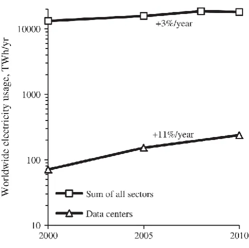
Data centres are massive facilities, which reportedly number more than 3 million worldwide and account for up to 1.5% of global electricity use (Fig. 1-1).

(20)

[image:20.595.188.437.68.316.2]

2

Figure 1-2. Variation of the global electricity usage compared to the sum of all sectors [1]

In a traditional air-cooled data centre a significant portion of this energy is used to cool the equipment so it does not overheat and fail. This poses huge opportunities for energy savings (Fig. 1-3).

(21)

3

Figure 1-3. Energy use breakdown and efficiently strategies for data centres (produced by Schneider Electric’s Data Centre Science Centre)

1.2

Impinging jets

Impinging jets have been used in many cooling/heating engineering applications, including cooling of electronic devices and turbine blades, de-icing of aircraft, and drying of textiles, among many others.

An impinging jet on a flat surface can be classified into different regions as specified in Fig. 1-4. In theory Schlichting et al. [3] and Jambunathan et al. [4] have defined them as follows:

 Potential core

This is the core of the jet which remains unaffected by the surrounding fluid; the velocity profile is identical to that of the jet exiting the nozzle and the turbulence intensity is low [5].

 Shear layer

(22)

4

Murray [5]-[6] and Schlichting et al. [1] demonstrate this proportional reduction in centreline jet velocity with the distance from the end of the potential core.

 Free Jet Region

The shear layer will continue to grow and develop as the jet moves further away from the nozzle eventually enveloping the potential core. This results in reduced jet velocity and increased turbulence intensity.

 Stagnation Zone

The stagnation point is the point where the mean velocity of the jet is equal to zero and there is a rise in static pressure. This region is also referred to as the deflection zone as it is here that the jet is deflected radially along the surface. This may also be referred to as the impingement region.

 Wall Jet Region

In this region the local jet velocity increases, resulting in a maximum jet velocity at the wall reducing proportionally to the distance from the wall. Due to the increase in turbulence caused by the shear layer between the ambient air and the wall jet, there is more heat transfer in this region. This increased turbulence makes its way to the boundary layer at the wall. Again, the entrainment of the ambient air causes this wall jet to expand and reduce in velocity, but increase in flow area.

(23)

5

Figure 1-4. Classification of distinct regions of an impinging jet on a flat surface (velocity vectors from CFD simulations results on an axisymmetric steady air jet;

chapter 4)

Impinging jets have been chosen as the basis of this study, due to their remarkable flow characteristics and their influence on heat transfer. To conduct a fundamental investigation of the complex fluid flow and heat transfer mechanisms of the jets, the first step is to perform a comprehensive review of the previous research studies performed in this field.

Stagnation Region

Free Jet Region

Shear Layer

Potential

Core

Ambient

Air

(24)

6

2

Literature Review

The present study focuses mainly on convective heat transfer of steady and unsteady jets, with an exclusive attention into the fluid mechanics of the jets. The emphasis is mainly on the development of the numerical model, and presenting detailed experimental results to allow for validation of the modelling technique.

Jet impingement is widely used in applications for high heat flux cooling like gas turbine blades and high-density electronic equipment, so its heat transfer performance has been the subject of many studies both numerically and experimentally in the last decades, [8]-[13].

2.1

Steady jets

(25)

7

evolution of vortices with distance from the jet exit has an influence on the magnitude of heat transfer coefficient along the wall. In another study [6], the same authors have shown that at low nozzle-to-target ratios (H ≤ 2D), secondary peaks in the radial heat transfer distributions are due to an abrupt increase in the turbulence in wall jet.

Thanks to the progress in computational performance, various numerical investigations have been performed to study the heat transfer coefficient distributions of impinging jet flows.

A number of numerical studies have qualitatively predicted the main flow features and heat transfer trends; however the results for local heat transfer distributions do not consistently produce acceptable quantitative agreement with experiments [14]-[15]. Furthermore, there are few studies recommending a reliable computational methodology for transitional jet impingement. This is the main motivation of the current study, which uses the established experimental methodologies of previous studies by the authors, O’Donovan and Murray [5]-[6] and Persoons et al. [13], for validation. As described by Caggese et al. [16], the inlet turbulence intensity has a strong effect on the heat transfer coefficient distribution, so the inlet turbulence profile must be chosen appropriately in order to fit the numerical model with experimental data. As will be described in section 4.1.1, the profiles of velocity and turbulence intensity exiting the nozzle are mapped from a separate model for the long inlet nozzle pipe to make the inlet boundary conditions more realistic.

(26)

8

parameter ranges and turbulence models used in some selected numerical studies from the literature. Different CFD models have been used, for a range of Re and H/D values (see Fig. 2-1).

Figure 2-1. Schematic diagram of steady impinging jet flow

Table 2-1.Overview of parameter ranges and turbulence models used in selected numerical studies

Re H/D Turbulence model

Draksler and Koncar [15] 20,000-23,000 1-2 SST

Caggese et al. [16] 16,500-41,800 0.5-1.5 SST

Hadziabdic and Hanjalic

[17] 20,000 2 LES

Cziesla et al. [18] 5,800 8-12 LES

Kubacki and Dick [19] 13,500-20,000 4-10 Hybrid RANS/LES

Impingement surface

Nozzle

Um= constant

L

Steady impinging jet flow

H D

Um

time

Um

(27)

9

In addition, when the simulation domain contains laminar, transitional and turbulent flows at the same time in different regions, the laminar-turbulent boundary layer transition should be modelled correctly. Although other numerical jet impingement studies typically use a fully turbulent model in the domain [16], an alternative is to employ a transition turbulence model called the Gamma-Theta model [20]-[22]. This model is based on two transport equations for intermittency and the transition momentum thickness Reynolds number, which determine the state of the boundary layer. The model becomes more useful in wall-bounded flows, in which the wall shear stress or the surface heat transfer rate are of interest. It is designed to predict the location and extent of laminar to turbulent flow transition which in turn significantly affects the heat transfer coefficient distribution. For impinging jet heat transfer at low values of nozzle-to-surface ratio (H ≤ 2D, O’Donovan and Murray [5]), the local increase in wall-normal velocity fluctuations

(28)

10

2.2

Pulsating jets

[image:28.595.138.503.359.670.2]

Steady impinging jets are considered as an effective technique to achieve convective heat transfer due to a very thin thermal boundary layer forced over a surface [5] and [24]. Pulsating or intermittent impinging jets, shown in Fig. 2-2, are generally believed to enhance heat transfer when compared to steady jets, although there remains a lack of consensus on the level of enhancement; for some conditions the heat transfer can even be impaired [25]-[33]. The intermittent nature of a pulsating jet effectively redevelops and breaks up the boundary layer within each pulsation period, which may result in a thinner boundary layer than that of an equivalent steady jet. This can be achieved using little additional energy with no need to increase the pressure or flow rate [25]. The shortening and spreading of the pulsating jet also allows for higher turbulence levels and promotes flow instabilities [29].

Figure 2-2. Schematic diagram of pulsating impinging jet flow

There is a lack of consensus in the scientific literature about the effect of flow pulsation on convective heat transfer enhancement. Although many studies have been carried out, the findings about the potential heat transfer enhancement induced by

Impingement surface

Nozzle

Um= f(time)

L

Pulsating impinging jet flow

H D

Um

time

Um

(29)

11

pulsating jets are quite varied [26]-[32]. Thus, some researchers report a significant heat transfer enhancement [26]-[29], while other studies reported no enhancement or even a reduction of the heat transfer using pulsating jet impingement [30]-[32]. Camci and Herr [26] found enhancement factors in stagnation heat transfer of up to 70% for Re = 14,000, H/D = 24, and f = 100 Hz (Sr = 0.033). Intermittent pulsation with a square-wave form has been experimentally investigated by Zumbrunnen and Aziz [27]; they reported significant heat transfer enhancement of up to 100% using the square-wave pulsation at high frequency f = 142 Hz (Sr = 0.37). Different waveform shapes were also investigated by Herwig and Middelberg [28], showing that a square-wave form pulsation produces much higher enhancement (for Sr = 0.08, 𝛿𝑁𝑢₀= 25%) than triangular or sinusoidal forms. The numerical results presented by Xu et al. [29] show that increase in the Reynolds number and pulsation frequency augments the Nusselt number compared to steady flow (up to 47%). In contrast, Liu and Sullivan [30] have measured changes in heat transfer due to pulsation of -10% to +10%, depending on the pulsation frequency and H/D. Using an acoustically excited air jet from a contoured nozzle, O’Donovan and Murray [31] have also reported a heat transfer reduction of up to -21% for 10,000 ≤ Re ≤ 30,000 and 0.5 ≤ H/D ≤ 2. This lack of consistency in findings is mainly due to the different ranges of parameters used in different investigations. Persoons et al. [24] have recently observed a change in behaviour due to flow pulsation in an axisymmetric impinging jet. Thus, for H/D=1 and a low pulsation frequency (Sr < 0.025), a reduction in stagnation point heat transfer rate by 13% is observed, increasing to positive enhancements for Sr.(H/D) > 0.1 up to a maximum enhancement of 48% at Sr (H/D) = 0.6.

(30)

12

(31)

13

2.3

Synthetic jets

A synthetic jet is typically generated from a partially closed cavity with an orifice and an oscillating diaphragm (see Fig. 2-3). Vibration of the diaphragm draws in and ejects ambient fluid through the orifice. This results in a train of vortex rings at the orifice outlet, to form the external jet flow. The train of vortex rings is able to entrain surrounding air into the high momentum jet core, resulting in increased flow controlling capabilities [13].

Figure 2-3. Schematic diagram of single synthetic jet flow

For an orifice diameter or slot width, D, the Reynolds number, Re = ρU0D/μ, and

stroke length, L0, govern the flow field of a free synthetic jet as defined by Smith and

Glezer [79]. The stroke length is defined as the distance that a slug of fluid travels away from the orifice during the ejection portion of the cycle Holman et al. [80]. The stroke length 𝐿₀ is defined as:

𝐿0 = 1

𝐴∫ ∫ 𝑣(𝑥, 𝑧, 𝑡) 𝑑𝐴 𝐴

1/(2𝑓)

0

𝑑𝑡 = 𝑈0 𝑓

(2-1)

The variables 𝑣(𝑥, 𝑧, 𝑡) and f are the instantaneous orifice velocity and the driving

frequency of the synthetic jet, respectively. 𝐴 is the cross-sectional area of the orifice. Vibrating

diaphragm Single synthetic jet flow

D

Um

L Um= f(time)

Um

0

time

(32)

14

Several applications of free synthetic jets in flow control techniques have been numerically and experimentally studied; for instance, applications in separation control by Zhang and Samtaney [81], Mittal and Rampunggoon [82], and Ozawa et al. [83], mixing enhancement by Jabbal and Zhong [84], Liu et al. [85], and Xia and Zhong [86], thrust-vectoring by Ibrahim and Skote [87] and virtual surface shaping by Mittal and Rampunggoon [82].

Furthermore, synthetic jets have become an interesting method of electronics cooling, resulting in continued research activities in this field. The local convective heat transfer of an impinging synthetic jet has been shown to rival that of a steady impinging jet as reported by Campbell et al. [88], Smith and Swift [89], Mahalingam [90] and Persoons et al. [13].The major advantage of synthetic jets is their zero net mass-flux nature, since the jets recycle the ambient fluid. Thus, the system does not require any additional components making synthetic jets advantageous for cooling in confined geometries, such as microelectronic thermal management.

Single synthetic jets have been experimentally investigated in various studies to date; see Smith and Glezer [79], Glezer and Amitay [91], Shuster and Smith [92], Valiorgue et al. [44], and Persoons et al. [13]. Persoons et al. [13] have provided an objective comparison of axisymmetric impinging synthetic jets versus steady jets through a wide range of operating conditions.

In addition to experimental investigations, several studies have used numerical modelling to understand the behaviour of synthetic jets. Provided the models are diligently validated, computational fluid dynamics can provide valuable additional information to better gain insight into the complicated nature of the fluid mechanics of synthetic jets.

2.3.1 Numerical investigations of single synthetic jet flows

(33)

15

to the complexity of their measurement; see Mohseni and Mittal [93]. Challenges and limitations associated with CFD modelling of synthetic jets have to contend with complex flow phenomena including flow separation, compressibility, unsteadiness, vortex dynamics and boundary layer formation.

Some numerical studies performed in this field have used an oscillating boundary condition at the exit of the orifice slot. This is done by setting an empirical harmonic function as the inlet velocity to the jet domain, 𝑈̅̅̅̅𝑖𝑛, defined as:

𝑈_𝑖𝑛

̅̅̅̅ = 𝑈_𝐴𝑓(𝜂) sin(2𝜋𝑓𝑡) (2-2)

where UA is the amplitude of the harmonic function, and 𝜂 is the cross-stream direction. These values are usually approximated using an experimental study performed at the corresponding parameter settings of the numerical model under investigation. The simplified inlet boundary condition (I.B.C.) truly reduces the amount of the complexity and the computational time during the solution procedure. However, this leads to an over-simplification of boundary conditions in the numerical model which is known to be the major challenge in this field of study. Table 2-2 summarizes a comprehensive overview of various numerical studies performed to evaluate single synthetic jets (S.J.). This table also points out the major features and characteristic parameters used by different studies, namely the configuration under investigation, stroke length (L0/D), Reynolds number (Re), actuation frequency (f), and method used for simulation. The latter represents two items: first the turbulence model used in each study and second the method practiced to simulate the dynamic flow phenomenon in the cavity, which can be either a simplified inlet boundary condition (I.B.C.) at the orifice slot or Dynamic Mesh (DM) scheme. Dynamic Mesh scheme has been used in a limited number of studies to date (see Table 2-2).

(34)

16

the essential features of the jet without modelling the detailed breakdown of the vortices or the details of the cavity flow.

Using the unsteady compressible Navier–Stokes equations, both the interior of the actuator cavity and the external jet flow field were investigated by Rizzetta et al. [95]. Both the spatial and temporal quality of the results were established via mesh-size and time-step studies. The internal results are generated with an overset deforming zonal mesh system, whereas the jet flow field is obtained by a high-order compact-difference scheme. A comparison is made with experimental data in terms of the mean and fluctuating components of the jet velocity. Simulations captured span wise instabilities that led to a breakup of the coherent vortex structure. They reported that with sufficient computational resources and complete knowledge of physical details of the actuating device, complex synthetic jet flow fields can be accurately simulated.

(35)

17

due to the misalignment of the strain and anisotropy tensors, is crucial. Therefore, linear eddy-viscosity models must be discarded for these types of pulsed flows, in particular for flow control using synthetic jets. Comparisons of long-time-averaged quantities are misleading because of the propagation of errors. When phase-averaged quantities are compared in detail, the deficiencies of linear eddy-viscosity models clearly appear. In order to evaluate the ability of the models to reproduce the unsteady dynamics of the flow, it is much more relevant to focus on the behaviour of the vortex dipole, in terms of location, intensity, convection velocity and penetration into the ambient fluid: the Reynolds-stress model is able to reproduce the correct dynamics, contrary to the k – ε. Rumsey et al. [97] arrived at the opposite conclusion reporting that linear eddy-viscosity models produce the best results among URANS models.

Rumsey et al. [97] have explored two different synthetic jet flows issuing into a turbulent boundary layer crossflow through a circular orifice. The use of URANS was shown to be appropriate for synthetic jet flows. The computations demonstrated good prediction of the qualitative behaviour of the synthetic jet flow field. However, quantitatively there were many specific differences. A major reason for the discrepancies between the URANS and the experimental results, was noted by the authors to be related to the time-dependent boundary condition which was applied at the centre of the orifice exit (simplified I. B. C.). They have finally emphasized the importance of including the region inside the cavity when modelling synthetic jets, and concluded that use of I. B. C. was an oversimplification that failed to capture the complex nature of the flow field near the orifice, particularly during the ejection phase of the cycle.

With an aim to develop a numerical predictive model for future designs of synthetic jet based active cooling substrates, Wang et al. [98]utilized a LES turbulence modelling scheme to perform the 3D simulations. To reduce the complexity of the model and the computational time of simulations, the vibration diaphragm boundary condition is simulated as a sine wave velocity boundary.

(36)

18

demonstrated that the compressibility of air is very significant. The effects of varying the frequency of the jet for a fixed pressure difference between the ends of the channel, and with a fixed jet Reynolds number, have been studied with air as the working fluid. The flow field results were not compared to experimental data in their study.

Ozawa et al. [83]have simulated the interaction between a synthetic jet and a laminar separation bubble caused by adverse pressure gradient in a boundary layer. In the numerical model including the synthetic jet actuator, the synthetic jet velocity at the exit of the cavity was defined as an input. To perform LES, a Dynamic Smagorinsky model was used for the sub-grid scale stress (SGS) terms. Their model was capable of capturing the basic features, including the transition from laminar to turbulent flow. However, simulating the transition from laminar to turbulent flow still remains a challenge.

The moving diaphragm can be modelled with a moving piston boundary condition as well as with a moving wall boundary condition. This is performed by Jain et al. [101]to investigate the effect of various cavity parameters on the ensuing synthetic jet flow, by use of a laminar flow model. It is observed that the approximations of the boundary condition in terms of a velocity inlet with a top hat profile or in terms of a sinusoidal moving piston do not simulate the actual behaviour of a vibrating diaphragm.

(37)

[image:37.595.100.527.90.623.2]

19

Table 2-2. Review of CFD studies for single synthetic jets

Configuration L0/D Re f (Hz) Method

Kral et al.

[94]

S. J. into

quiescent air 2.7 – 16.5* 500 – 3,000 1,000

I. B.C.

Spalart-Allmaras

Rizzetta et al.

[95]

S. J. actuator 4.1 – 8.2* 750 – 1,500 1,000

D. M.

DNS

Carpy and

Manceau

[96]

S. J. into

quiescent air

29.7* 2,400 444.7

I. B.C.

URANS

Wang et al.

[98]

S. J. based active

cooling substrates

- 600 -

I. B.C.

LES

Rumsey et al.

[97]

S. J. in crossflow - - 24 - 150

I. B.C.

URANS

Timchenko

[99]

S. J. in

micro-channels

18.9 -

56.7*

103 10 - 30 D. M.

Laminar Model

Ozawa et al.

[83]

S. J. for active

flow control

27.5* 500 100 I. B. C.

LES

Jain et al.

[101] Axisymmetric S. J.

0.83 –

42.5* 167 – 1,544 200 – 1,100

I. B.C. & D. M.

Laminar Model

Harinaldi and

Rhakasywi

[103]

Impinging S. J. 48.8 – 195* 1,421 - 2,843 80 - 160

I. B. C.

SST

Silva and

Ortega

[104]

Impinging S. J. 2.33 - 6.9* 508 400 – 1,200

I. B. C.

Laminar Model

Bazdidi-Tehrani

et al. [102]

Impinging S. J. 0.55 – 27.6 2210 30 - 2500 I. B. C.

V2_{-f Model}

Xia et al.

[105]

S. J. at low

Reynolds numbers 0.52 - 11.1 14.8 – 553 2 - 10

I. B. C.

Laminar Model

(38)

20

Due to the limitations of piezoelectric material, it has been hard to modify the controlling efficiency of small-scale synthetic jet actuators for the limited maximum amplitude. A high-power synthetic jet actuator can fulfil the efficiency and power requirements of full-scale flow control applications; see Liu et al. [85]. However, the newly designed actuators are not compact enough to be utilized conveniently into high-density electronic equipment and other devices. To meet the “strength” and “micro-” requirements in various applications, it is necessary to investigate the optimization design methods of adjacent synthetic jets actuators; see Ritchie and Seitzman [106].

2.3.2 Numerical investigations of adjacent synthetic jet flows

The strong entrainment of the surrounding flow which is induced by the jet in the vicinity of the cavity outlet can be used to dynamically vector the jet. A pair of side-by-side synthetic jets can form a larger jet, as experimentally studied by Smith and Glezer [78]. They have studied two adjacent synthetic jets 0.5 mm wide placed apart from each other. Their results show that if the jets are in phase, the inner vortices cancel each other, resulting in a single merged jet. The combined jet has stronger controlling ability compared with a single synthetic jet. When one of the jets is leading in phase, its vortex pair and the suction effect from the adjacent jets deflects the vortex pair directions and the merged jet is vectored toward the actuator leading in phase. The relative phase difference of the jet actuators can be used to manipulate the merged jet which results in a great effect on the controlling ability of the synthetic jet actuator.

(39)

21

jet. This effect prevents recirculation of heated fluid to the cavity without the need for an external cross-flow (e.g. driven by a fan) and was shown to enhance the convective heat transfer performance of the jet pair. Heat transfer and PIV measurements by Persoons et al. [108] suggest an optimum phase difference region of 90° < 𝛿∅ < 120° for constant values of Re = 300, L0/D = 29 and an orifice-to-orifice centre separation S = 3D. In this range of phase difference an effective cross-flow was set up whilst maintaining strong vortex mixing at impingement, resulting in the highest convective heat transfer rates. Using PIV and infrared thermography Fanning et al. [109] have recently presented a wide range of heat transfer measurement and discussed the mechanism of cross-flow induced by the out-of-phase synthetic jets.

A very limited number of studies have considered interaction of a pair of adjacent twin jets. This becomes the case especially when the major focus is on the effect of phase difference between adjacent cavities on vectoring of the merged jet. A summarized overview of numerical studies performed to evaluate adjacent synthetic jets is presented in Table 2-3.

In the study of Guo et al. [110], the cavity geometry is included in the simulations and the actuator boundary conditions using Eq. (2-2) are applied at the bottom of the two cavities. RANS equations are solved to simulate the interaction of two adjacent synthetic jet actuators. Cases with different relative phases between the adjacent jets are simulated. For a phase difference of 130°, the vortex pairs generated by the blowing strokes of the two jets are both vectored towards the left wall even before they separate from the jets, and travel away from the synthetic jets along the wall anddissipate gradually. They have also noted that for relatively higher phase differences between two jets, the direction of the merged jet is sensitive to the initial phases.

(40)

22

Luo et al. [107] have investigated a novel piezoelectric-driven actuator. Synthetic jet actuator is composed of two emitting slots, two sealed cavities bounded on one end by a single PZT diaphragm, and a slide block. This can be regarded as a pair of adjacent jets with a constant phase difference of 180 ͦ. The study mainly focuses on introducing the adjustable actuator design. The numerical results are based on an I. B. C. and 𝑘 − 𝜀

model are only limited to velocity contours of flow field into quiescent air, without a comparison to experiments. The same turbulence model and boundary condition is used by Liu et al. [85] to evaluate the mechanism of adjacent synthetic jets and the influence of phase difference on the mixing of coaxial jets. Their results indicate that a phase difference between the jets can lead to reduced vortex size, reduced vortex strength to a greater degree, and finally, decreased controlling ability. The unsteadiness mainly results from the vortex-vortex interaction and energy exchange, and the detailed mechanism needs further investigation in the future.

(41)

[image:41.595.114.521.92.320.2]

23

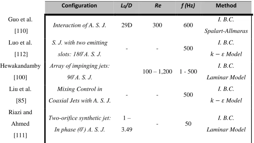
Table 2-3. Review of CFD studies for adjacent synthetic jets

Configuration L0/D Re f (Hz) Method

Guo et al.

[110] Interaction of A. S. J. 29D 300 600

I. B.C.

Spalart-Allmaras

Luo et al.

[112]

S. J. with two emitting

slots: 180̊ A. S. J. - - 500

I. B.C.

𝑘 − 𝜀 Model

Hewakandamby

[100]

Array of impinging jets:

90̊ A. S. J. 100 – 1,200 1 - 500

I. B.C.

Laminar Model

Liu et al.

[85]

Mixing Control in

Coaxial Jets with A. S. J.

- - 500

I. B.C.

𝑘 − 𝜀 Model

Riazi and

Ahmed

[111]

Two-orifice synthetic jet: In phase (0̊ ) A. S. J.

1 –

3.49

- 50

I. B.C.

Laminar Model

Notes: I. B. C. = Inlet boundary condition, A. S. J. = Adjacent Synthetic Jets

To the best of our knowledge, there has not been an effort thus far to integrate the oscillating diaphragm motion in the simulation of a pair of adjacent synthetic jets and which is accompanied with experimental validations.

The complicated vortex structures in shear layer must be accurately calculated in order to understand the vortex-vortex and vortex-wave interactions which are difficult to understand. The intricate mechanism of adjacent synthetic jets and the effect of phase difference on vectoring of the merged jet is the major focus in this study.

As discussed above, the simulation of the actuator diaphragm is still a crucial challenge in the numerical modelling of synthetic jets which is overlooked in a lot of studies (see Table 2-2 and Table 2-3).

(42)

24

will be automatically updated inside the model without any need to modify the empirical boundary condition, shown in Eq. (2-2).

Alimohammadi et al. [38] have previously shown that the CFD model can reliably predict the fluid flow and heat transfer to steady and pulsating impinging jets for an extensive range of operating conditions. To predict the fluid flow behaviour of synthetic jets using numerical modelling, the previously validated transient numerical model for pulsating impinging jets [38] is extended to synthetic jets. This is done for both single jets and a pair of adjacent jets, considering the case of jets inssuing into quiescent air. This model is designed so as to overcome the previously described deficiency in the numerical modelling of synthetic jets. The oscillating wall of the cavity is simulated in the new model by means of dynamic mesh techniques. The results are compared to the results reported by Smith and Glezer [78], Persoons et al. [108], and Fanning et al. [109] and a set of experimental data obatined in this study on adjacent synthetic jets using Particle Image Velocimetry (PIV) techniques.

(43)

25

3

Research Objectives and Outline

3.1

Research objectives

This work aims to develop an experimentally validated numerical model for a wide range of jet flows for heat transfer applications in a progressive manner.

The main objectives of this study are the following:

• Verification of a computational fluid dynamics model to predict the fluid flow & heat transfer of steady and unsteady impinging jets, using detailed experimental measurements for validation.

• The effect of Reynolds number, jet-to-surface distance, nozzle diameter, pulsation frequency on heat transfer enhancement for pulsating jets.

• Quantification of the stagnation and area-averaged heat transfer enhancements achieved by flow pulsation.

• Proving an insight into the near-wall behaviour in the viscous sublayer to realize the governing heat transfer mechanisms.

• A full simulation of the internal flow in the jet cavities, as well as the external jet flow, for a pair of adjacent synthetic jets, using dynamic mesh techniques.

(44)

26

3.2

Thesis outline

Steady, pulsating and synthetic jets are three important manifestations of jet flows suitable for electronics cooling and thermal management applications, each having their own specific challenges to model numerically. This is mainly represented in chapters 4, 5 and 6, for steady, pulsating, and synthetic jets, respectively. Each chapter attempts to show the step-by-step procedure to extend the numerical model for each specific case. Every chapter includes the required descriptions about the numerical and experimental methodologies together with validation of CFD model for each specific case (e.g. steady jets, pulsating jets, synthetic jets). This is accompanied by a specific results and discussion section for each chapter and also a conclusion which bridges each chapter to the next one.

The remainder of this thesis is organised as follows:

Chapter 4 aims to establish and verify a robust RANS (Reynolds-averaged Navier-Stokes) computational fluid dynamics (CFD) methodology to accurately predict the local heat transfer coefficient for a circular steady impinging jet, using our own detailed experimental measurements for validation. The main goal is to capture the transition to turbulence in the wall jet and to ensure the model is valid over a wide range of operational and geometrical parameters, while keeping the computational cost low. This chapter is the first step towards a robust numerical methodology for unsteady impinging flows such as pulsating and synthetic jets ([13], [34]-[38]).

(45)

27

Following rigorous experimental validation, the CFD model is used as a stable tool to simulate operating conditions beyond the frequency range for reliable operation of the experimental pulsating valve. This shows how the numerical model helps the investigation to be extrapolated to much higher frequency jets.

As another motivation in this research, to better understand the potential heat transfer enhancement introduced by the flow pulsation, some of the effective near-wall flow characteristics, namely the radial velocity gradient, the normal vorticity, and the Reynolds stress components, are monitored. This approach reveals that these flow characteristics are directly proportional to the heat transfer distribution of steady and pulsating jets over the impingement surface, and shows the variation of jet frequency itself can affect the enhancement.

Chapter 6 reports the numerical and experimental study performed on synthetic jets.

The formation, evolution and interaction of a pair of adjacent synthetic jets is investigated numerically using computational fluid dynamics and experimentally using particle image velocimetry techniques. Both jet actuators are operated at the same condition but with an adjustable phase difference. The investigation considers a jet pair issuing into quiescent air. Simulation of full jet cavity incorporating the diaphragm motion is performed using Mesh Deformation techniques.

The effect of phase difference between the pair of adjacent synthetic jets on the vectoring of the merged jet is investigated. This leads to a better understanding of the fluid mechanics of adjacent synthetic jets and delivers a theoretical basis to be used in the future for their application.

Chapter 7 highlights the main conclusions of this study, considering the incremental

progression of complexity in the flow configurations from steady jets to pulsating jets and finally a pair of adjacent synthetic jets. This is done apart from the conclusion sections which are reported at the end of each chapter linking the findings to the next chapter.

(46)

28

4

Steady Impinging Jet Flows

(47)

[image:47.595.139.503.66.378.2]

29

Figure 4-1. Schematic diagram of steady impinging jet flow

4.1

Numerical methodology

For the numerical simulation of jet impingement, the commercial tool ANSYS CFX 14 is employed. This package uses an element-based finite volume method. This is done by integrating and discretising conservation equations, namely continuity, momentum and energy equations, plus the appropriate turbulence equations according to the selected turbulence model as a closure [39]-[40]. CFX uses a vertex-centred solver, so the solution variables are stored at the mesh vertices (nodes). To describe the way a variable changes across each element, solution fields and gradients at integration points are approximated using finite-element shape function. Likewise, following the standard finite-element approach, shape functions are used to evaluate spatial derivatives for the diffusion terms. The resulting linear system of equations that arises by applying the finite volume method to all elements are discrete conservation equations, which are solved using a coupled solver to reduce the number of iterations for convergence.

Attention is focused on the near-wall region since it is the most important for convective heat transfer. Some previous studies on heat transfer to impinging jets only

Impingement surface

Nozzle

Um= constant

L

Steady impinging jet flow

H D

Um

time

Um

(48)

30

qualitatively predict the flow physics, with a limited degree of quantitative accuracy for the solution of the energy equation which is closely linked to the convective heat transfer. The current chapter aims to improve the accuracy of heat transfer simulations by validating the results via comparison with experimental local heat transfer coefficient data (see Sections 4.2, 4.3 and 4.4).

4.1.1 Computational domain: geometry and boundary conditions

Figure 4-2 displays the two-dimensional axisymmetric computational domain and mesh used in the simulation of an unconfined round jet impinging on a flat plate. The dimensions are identical to that of the experimental setup used for validation (see Section 4.2.1). An assumption of axisymmetric flow in the domain provides a good approximation while saving time to achieve a satisfactory convergence (Alimohammadi et al. [37]), as verified by the comparison of CFD to experimental results presented in sections 4.3 and 4.4. The computational domain extends far enough from the area of interest (up to a radial distance of 16D from the jet centreline) to prevent outlet boundary effects on the results.

(49)

31

Figure 4-2. Computational domain, boundary conditions

The turbulence intensity at the domain inlet is also determined by means of the same mapping procedure of profiles obtained for the turbulent kinetic energy from a separate simulation. However, it should be noted that the turbulence intensity value at the nozzle inlet, remains unknown at this stage; the procedure to estimate the averaged turbulence intensity at the nozzle pipe inlet is described in section 4.3.5.

At the radial outlet and unconfined top boundaries of the domain, as the far-field boundaries which are free to the environment, an opening boundary condition with a constant temperature of 25 °C and zero relative pressure is used to allow the flow to leave and re-enter the domain, thereby enabling potential flow re-circulation. The planar heated wall surface at the bottom of the domain is set to a constant temperature of 60 °C, in agreement with the experiments (see Section 4.2.1).

4.1.2 Mesh generation

(50)

32

4-3); afterwards, it is refined and adapted iteratively in regions with large velocity, pressure, temperature and turbulence gradients in order to attain a stable solution. To have a computationally efficient model in low-gradient regions a coarse mesh scheme is applied, resulting in better control on the physical distance of the first grid point from the wall (y+_{). The adequate value of near-wall cell thickness is ensured by keeping the y}+

below unity for the near-wall cells.

Figure 4-3. Mesh used in the simulation of the unconfined axisymmetric impinging jet

Additionally, at least ten nodes are applied inside the viscous sub-layer within a small distance from the wall (of the order of 10-6_×_{D for the present problem). The final grid is}

generated to have a larger concentration of nodes close to the impingement wall and the jet mixing region, which take places between the jet and the surrounding entrained air. Section 4.3.1 shows the details of five different mesh sizes used for the grid independency study and their effect on heat transfer results.

4.1.3 Fluid properties

Fluid compressibility is negligible in the current problem since the local Mach number does not exceed 0.05. However since temperature differences of up to 35 °C may occur in the domain, a moderate change in air properties can be expected. A linear property table is employed to calculate the density, viscosity and thermal conductivity for the range of 25 °C to 60 °C in the domain, to include the effect of compressibility and changing fluid properties. As a result, the difference between the heat transfer results

(51)

33

extracted from incompressible and compressible models for the applicable range of Re numbers in this study (between 6000 and 14,000) is calculated to be less than 1%.

The relative importance of buoyancy forces (natural convection) due to the temperature variations in a mixed convection flow can be estimated using Richardson number (Ri) the ratio of Grashof number to the squared Reynolds number, which is proportional to the domain length scale. Due to the small length scale of the domain (with a maximum of 0.1 m, approximately), the maximum value of this ratio for the current problem is of the order of 0.002. Thus, buoyancy is neglected in the simulation.

4.1.4 Turbulence modelling and governing equations

As observed in impinging jet flow experiments, both laminar and turbulent flow occurs simultaneously in different regions. For laminar flow, the numerical solution of the momentum and continuity equations with a suitable grid is sufficient to resolve the flow phenomenon (see section A.4.2), but for turbulent or transitional flows, a turbulence model is required. Turbulence strongly affects the important global features of the flow, so the accurate and reliable prediction of turbulent flow phenomena is essential.

The decision regarding the appropriate model for simulations of turbulence in the domain is based on the flow physics and computational requirements depending on the generated grid and accuracy. Due to the boundary layer separation, a wall function is not an appropriate method to resolve the boundary layer [17]. Instead, directly resolving the boundary layer can provide accurate results. One of the major considerations is generating a near-wall mesh which is fine enough to resolve the laminar part of the boundary layer (viscous sub-layer) over a very small distance from the wall. The RANS turbulence models are broadly used in practical modelling for suitable accuracy and efficiency. The RANS turbulence models evaluated in the present study are: k-, RNG

k-, k-, and SST with and without a transition model. Section 4.3.6 describes the effect of

the different turbulence models on the results and the procedure for selection of an appropriate turbulence model in comparison with experimental data.

(52)

34

appropriate turbulence equations according to the final selected turbulence model (SST, as will be described in section 4.3.6) as a closure [40]. In addition, the present study employs an accurate and realizable laminar-turbulent transition model called Gamma-Theta model (-Re). This model employs new empirical correlations developed by Langtry and Menter [16-18], which have been broadly validated to work with the SST turbulence model.

Firstly, the transport equations for turbulent kinetic energy (k) and its specific dissipation rate () of the modified SST model to work with the -Re transition model are as follows ([20]-[22]):

𝜌𝐷𝑘 𝐷𝑡 =

𝜕

𝜕𝑥_𝑗[(𝜇 + 𝜎𝑘𝜇𝑡) 𝜕𝑘

𝜕𝑥_𝑗] + (𝛾𝑒𝑓𝑓𝜇𝑡𝑆

2_{− 𝜌𝑘}𝜕𝑢𝑗 𝜕𝑥_𝑗)

− 𝑚𝑖𝑛[𝑚𝑎𝑥(𝛾𝑒𝑓𝑓, 0.1), 1]𝜌𝛽∗𝜔𝑘

(4-1)

𝜌𝐷𝜔 𝐷𝑡 =

𝜕

𝜕𝑥_𝑗[(𝜇 + 𝜎𝜔𝜇𝑡) 𝜕𝜔

𝜕𝑥_𝑗] + 𝛼 (𝜇𝑡𝑆

2_{− 𝜌𝑘}𝜕𝑢𝑗

𝜕𝑥_𝑗) − 𝜌𝛽𝜔 2

+ 2𝜌(1 − 𝐹1)𝜎𝜔2 1 𝜔 𝛿𝑘 𝛿𝑥𝑗 𝛿𝜔 𝛿𝑥𝑗 (4-2)

where 𝑢𝑗 is the velocity vector, 𝜇 is the molecular viscosity, 𝜌 is the density, 𝑆 is the

strain rate tensor modulus and 𝛾𝑒𝑓𝑓 is the effective intermittency. Note that the

production term in the transport equation of  is not amended. The turbulent viscosity (𝜇𝑡) is defined as:

𝜇_𝑡 = 𝜌𝑘𝑇, 𝑇 = 𝑚𝑖𝑛 [ 1

𝑚𝑎𝑥 [𝜔, 𝑆𝐹₂/𝑎₁], 0.6

√3𝑆]

(4-3, 4-4) the functions 𝐹1 and 𝐹2 are calculated as:

𝐹₁ = max[𝐹₃, 𝑡𝑎𝑛ℎ(𝑎𝑟𝑔₁4)] ,

𝑎𝑟𝑔₁ = 𝑚𝑎𝑥 [𝑚𝑖𝑛 ( √𝑘 0.09𝜔𝑦 ,

500𝜐 𝜔𝑦2) ,

2𝑘 𝑦2_𝐶𝐷

𝑘𝜔 ]

(4-5, 4-6)

𝐶𝐷_𝑘𝜔 = 𝑚𝑎𝑥 (1 𝜔

𝛿𝑘 𝛿𝑥_𝑗

𝛿𝜔

(53)

35

𝐹₂ = 𝑡𝑎𝑛ℎ(𝑎𝑟𝑔₂2_), _𝑎𝑟𝑔

2= 𝑚𝑎𝑥 ( 2√𝑘 0.09𝜔𝑦 ,

500𝜐 𝜔𝑦2)

(4-8, 4-9)

𝐹₃ = 𝑒𝑥𝑝 (− (𝑅𝑦 120)

8

) , 𝑅_𝑦 = 𝜌𝑦𝑘1/2/𝜇 (4-10,

4-11) where 𝑦 is the normal distance from the nearest wall, and 𝑅_𝑦 is wall-distance based turbulent Reynolds number. The coefficient 𝜙, which is a general term for 𝜎_𝑘, 𝜎_𝜔, 𝛽 and

𝛼 in the equations (4-1) and (4-2), is estimated from the blending function (𝐹₁) as follows:

𝜙 = 𝐹₁𝜙₁+ (1 − 𝐹₁)𝜙₂ (4-12)

where the coefficients 𝜙1, 𝜙2 are:

𝜎_𝑘1= 0.85, 𝜎_𝜔1= 0.65, 𝛽₁ = 0.075, 𝛼₁ = 𝛽₁/𝛽∗_{− 𝜎}

𝜔1𝜅2/√𝛽∗

𝜎_𝑘2= 1.0, 𝜎_𝜔2 = 0.856, 𝛽₂= 0.0828, 𝛼₂ = 𝛽₂/𝛽∗− 𝜎_𝜔2𝜅2/√𝛽∗

and 𝑎₁ = 𝑓0.3, 𝜅 = 0.41, 𝛽∗= 0.09.

The -Retransition model is made of two transport equations for the intermittency () and the transition momentum thickness Reynolds number (𝑅̃𝑒_𝜃𝑡) which are written as follows ([20]-[21]):

𝜌𝐷𝛾 𝐷𝑡 =

𝜕

𝜕𝑥_𝑗[(𝜇 + 𝜇𝑡 𝜎_𝛾)

𝜕𝛾

𝜕𝑥_𝑗] + 𝐹𝑙𝑒𝑛𝑔𝑡ℎ𝑐𝑎1𝜌𝑆(𝛾𝐹𝑜𝑛𝑠𝑒𝑡)

0.5_{(1 − 𝑐} 𝑒1𝛾)

+ 𝑐_𝑎2𝜌Ω𝛾𝐹_{𝑡𝑢𝑟𝑏}(1 − 𝑐𝑒2𝛾)

(4-13)

𝜌𝐷𝑅̃𝑒𝜃𝑡

𝐷𝑡 =

𝜕 𝜕𝑥𝑗

[𝜎𝜃𝑡(𝜇 + 𝜇𝑡) 𝜕𝑅̃𝑒_𝜃𝑡

𝜕𝑥𝑗

] + 𝑐𝜃𝑡 (𝜌𝑈)2

500𝜇 (𝑅𝑒𝜃𝑡− 𝑅̃𝑒𝜃𝑡)(1 − 𝐹𝜃𝑡) (4-14)

(54)

36

The above described controller functions are written as:

𝐹_{𝑜𝑛𝑠𝑒𝑡} = 𝑚𝑎𝑥(𝐹_{𝑜𝑛𝑠𝑒𝑡2}− 𝐹_{𝑜𝑛𝑠𝑒𝑡3}, 0) (4-15)

𝐹_{𝑡𝑢𝑟𝑏} = 𝑒𝑥𝑝[−(𝑅_𝑇/4)4_] _(4-16)

𝐹_{𝑜𝑛𝑠𝑒𝑡2} = 𝑚𝑖𝑛[max(𝐹_{𝑜𝑛𝑠𝑒𝑡1}, 𝐹_{𝑜𝑛𝑠𝑒𝑡1}4) , 2] (4-17)

𝐹_{𝑜𝑛𝑠𝑒𝑡1} = 𝑅𝑣

(2.193𝑅𝑒_𝜃𝑐)

(4-18)

𝐹𝑜𝑛𝑠𝑒𝑡3 = 𝑚𝑎𝑥 (1 − (

𝑅_𝑇 2.5)

3

, 0) (4-19)

𝐹_𝜃𝑡 = 𝑚𝑖𝑛 {𝑚𝑎𝑥 [𝐹_{𝑤𝑎𝑘𝑒}. 𝑒𝑥𝑝 [− ( 𝑈 2

375Ω𝑣𝑅̃𝑒_𝜃𝑡) 4

] , 1 − (𝑐𝑒2𝛾 − 1 𝑐_𝑒2− 1 )

2 ] , 1}

(4-20)

𝐹_{𝑤𝑎𝑘𝑒} = 𝑒𝑥𝑝[−(𝑅_𝜔/105₎2_]

(4-21)

𝑅𝑣 = 𝜌𝑆𝑦2

𝜇 , 𝑅𝑇 = 𝜌𝑘

𝜇𝜔, 𝑅𝜔 = 𝜌𝜔𝑦2

𝜇

(4-22, 4-23, 4-24)

where 𝑅_𝑣 is the strain-rate Reynolds number, 𝑅_𝑇 is a turbulent Reynolds number (generally known as the viscosity ratio). 𝑅𝑒𝜃𝑐 is the critical momentum th

A validated computational fluid dynamics methodology for characterisation of fluid flow and heat transfer in unsteady jets