Composite likelihood inference for hidden Markov models for dynamic networks

Munich Personal RePEc Archive

Composite likelihood inference for hidden

Markov models for dynamic networks

Bartolucci, Francesco and Marino, Maria Francesca and

Pandolfi, Silvia

14 October 2015

Online at

https://mpra.ub.uni-muenchen.de/67242/

Composite likelihood inference for hidden Markov models for

dynamic networks

Francesco Bartolucci Department of Economics University of Perugia (IT) E-mail: [email protected]

Maria Francesca Marino Department of Economics University of Perugia (IT)

E-mail: [email protected]

Silvia Pandolfi Department of Economics University of Perugia (IT) E-mail: [email protected]

October 14, 2015

Abstract

We introduce a hidden Markov model for dynamic network data where directed relations among a set of units are observed at different time occasions. The model can also be used with minor adjustments to deal with undirected networks. In the directional case, dyads referred to each pair of units are explicitly modelled conditional on the latent states of both units. Given the complexity of the model, we propose a composite likelihood method for making inference on its parameters. This method is studied in detail for the directional case by a simulation study in which different scenarios are considered. The proposed approach is illustrated by an example based on the well-known Enron dataset about email exchange.

Keywords: Dyads; EM algorithm; Enron dataset; Latent Markov models

1

Introduction

A number of social and biological phenomena can be naturally represented in terms of networks. Here, the connection between units, that is, “actors” or “nodes”, is the main target of inference.

On these grounds, in the last decades, statistical models for the analysis of this type of data have known a flowering interest. Most research has focused on static networks, where data

(2010) for a review. However, in some cases, the research interest may concern the evolution

of networks over time. The Enron dataset (Klimt and Yang, 2004) on email exchange between employees of the company gives an interesting empirical example. Here, one may be interested

in understanding how email traffic evolves over time.

In this context, standard tools of analysis need to be extended to deal with observations repeatedly taken over time, that is, with multiple snapshots of the network observed at different

time points. Thus, the analysis falls into the context of longitudinal data analysis. As it is well known, although repeated measurements allow us to get deeper information on the phenomena of

interest, the dependence between measures taken on the same sample units represents a further challenge that has to be faced (e.g., Diggle et al., 2002). Recently, there has been a growing

amount of work on analysing dynamic networks. Key contributions are represented by dynamic exponential random graph models (Robins and Pattison, 2001) and continuous latent space

models (Sarkar and Moore, 2005; Sarkar et al., 2007; Hoff, 2011; Lee and Priebe, 2011; Durante and Dunson, 2014). Within this latter context, network edges are projected in a reduced latent

space where edge relations are explored.

An alternative class of models focuses on clustering nodes. Stochastic Block Models (SBMs;

Holland and Leinhardt, 1976) assume that network nodes belong to one of k distinct blocks. These are defined by a discrete latent variable, with the probability of observing a connection

between two nodes only depending on the corresponding block membership. That is, units in the same block connect to all the others in a similar fashion and are said to be stochastically

equivalent. These models offer a concise description of the network, as a possible large number of connections is summarised by the connections between the blocks to which the units belong.

Yang et al. (2011) extended standard SBMs by considering time-varying block memberships for each unit that evolve over time according to an unobservable Markov chain. The resulting

model can be conceived as a particular kind of hidden Markov model (for general references, see Zucchini and MacDonald, 2009; Bartolucci et al., 2013) for dynamic networks. Xu and Hero

(2014) further extended the dynamic SBM of Yang et al. (2011) by considering time-varying edge probabilities, while Xu (2015) proposed an approach in which the presence of an edge at a

given occasion directly influences future edge probabilities. An approach that is in between the dynamic latent space and the dynamic SBM is the dynamic mixed-membership SBM by Xing

In the framework of static networks, a number of statistical models for dyadic mutual

depen-dences have been defined; in this context,reciprocal relations between units are the main target of inference. To the best of our knowledge, these types of relation have not been deeply investigated

for dynamic networks. Avoiding restrictive assumptions about the dependence/independence between reciprocal relations turns out to be crucial in order to ensure model flexibility.

Here, starting from the proposal by Yang et al. (2011), we develop a SBM for dynamic

networks, observed in discrete time, in which the unit of analysis is thedyad. As opposed to the Bayesian approaches suggested in the above mentioned works which are all based on MCMC

algorithms, we obtain parameter estimates in a maximum-likelihood perspective. In this respect, a reduced computational effort is required and assumptions on the prior distribution of the model

parameters can be avoided. In particular, in order to overcome the intractability of the observed data likelihood, we propose a composite likelihood approach (Lindsay, 1988; Cox and Reid, 2004)

that consistently simplifies the estimation procedure and leads to reliable parameter estimates. The implementation of this method is based on an Expectation-Maximisation algorithm (EM;

Dempster et al., 1977) implemented using the standard Baum-Welch recursions (Baum et al., 1970). For a related approach we refer to Bartolucci and Lupparelli (2015) who dealt with

composite likelihood inference for hidden Markov models but in a different context, which is that of multilevel longitudinal data without a social network perspective. The proposed composite

likelihood estimation method is studied via simulation and through the application to the Enron dataset, which represents a benchmark in the dynamic network literature. Upon request, we

make available to the reader ourR_{implementation of the algorithm.}

The paper is organised as follows. Section 2 introduces the dynamic SBM, while Section 3

entails the description of the algorithm for parameter estimation. The results of the simulation study and of the real data application are provided in Sections 4 and 5, respectively. Last section

gives some concluding remarks and outlines potential future developments.

2

The dynamic stochastic blockmodel

Let Y(_ijt) = (Y_ij(t), Y_ji(t))′ _{denote the random vector corresponding to the dyad recorded at time}

units in the network remain unchanged during time. Also, we denote by ˜Yij = (Y(1)ij , . . . ,Y

(T)

ij )

the matrix of dyadic relations between iand j observed during the analysed time window. As usual, realisations of random variables and related objects will be denoted by lower case letters,

so that, for instance, y_ij(t) is the observed value of Y_ij(t). Finally, we define the set of all network snapshots taken across time asY ={Y(_ijt), i= 1, . . . , n−1, j=i+ 1, . . . , n, t= 1, . . . , T}.

In this paper, we focus ondirected networks, where the existence of an edge from unitito unit

jat a given occasion does not imply an edge fromjtoi. The extension to the undirected case is straightforwardly obtained with minor changes to the estimation algorithm. A typical example of directed networks is that of friendship nominations, where relations are not necessarily mutual,

or that of email exchange that is object of the present paper; see Section 5. In this context, the dyadic relation betweeniand jcan be eithernull (“00”),asymmetric (“01” or “10”), ormutual

(“11”).

In the spirit of dynamic SBMs, we assume the existence of a hidden (or latent) Markov

chainUi = (U_i(1), . . . , U_i(T))′ for each sample unit i, which is defined over the finite state space

{1, . . . , k}. Latent processes Ui, i = 1, . . . , n, are assumed to be mutually independent and

identically distributed, with initial probability vectorλ= (λ1, . . . , λk)′and transition probability

matrix Λ _{of dimension k×k with elements λu|v. The elements of this vector and matrix are}

defined as

λu = p(U_i(1)=u), u= 1, . . . , k,

λu|v = p(Ui(t)=u|U

(t−1)

i =v), u, v= 1, . . . , k, t= 2, . . . , T.

Note that these parameters are assumed to be constant over time and shared by all units in the network. These assumptions are seldom restrictive, even if generalisations are easily obtained

by introducing unit and time-dependent covariates in the model; see Bartolucci et al. (2013) for a thorough discussion on the topic.

Concerning the relations between the units in the network, we assume the following model specification. For a givent= 1, . . . , T,the dyadY(_ijt)only depends on the latent states occupied by units i and j at occasion t, that is, U_i(t) and U_j(t). Given these latent variables and for

other dyad and the corresponding probabilities are defined as

ψ_y1y2|u1u2 =p(Y_ij(t) =y1, Yji(t)=y2 |Ui(t)=u1, Uj(t) =u2), u1, u2 = 1, . . . , k, y1, y2 = 0,1. (1)

That is, conditional on the states occupied by units in the dyad (U_i(t) = u1, U_j(t) = u2) at a given time occasion, the following 2×2 matrix, denoted by Ψ_{(u), completely describes the}

corresponding dyadic relation ❍

❍ ❍

❍ ❍

❍ ❍

❍❍

Yij

Yji

0 1

0 ψ_00|u1u2 ψ_01|u1u2 ψ_0·|u1

1 ψ10|u1u2 ψ11|u1u2 ψ1·|u1

ψ·0|u2 ψ·1|u2 1

It is worth noticing that a different way to describe the model introduced so far is by

assuming that the dyad Y(_ijt), for each i < j, follows a bivariate hidden Markov model defined on an augmented state space. In detail, let ˜Uij = (U(1)ij , . . .U

(T)

ij ) be the augmented hidden

Markov process with k2 states denoted byu, whereU(_ijt) = (U_i(t), U_j(t))′ and u= (u1, u2)′. The corresponding initial and transition probabilities are completely defined by the parameters of

the univariate latent process Ui according to the following expressions

πu=p(U(1)_ij =u) =λu1λu2,

πu|v =p(U

(t)

ij =u|U

(t−1)

ij =v) =λu1|v1λu2|v2,

wherev = (v1, v2)′ stands for the latent state at the previous occasion. In a more compact form, the quantities above can be directly obtained as π=λ⊗λand Π₌Λ_⊗Λ_{, where ⊗ denotes}

the Kronecker product. As it is standard in the Markov model literature, due to the Markovian property, the marginal distribution of the augmented latent process is given by

p( ˜Uij = ˜u) =πu(1)

T

Y

t=2

π_u(t)_|u(t−1),

analysed time window is given by

p( ˜Yij = ˜y|U˜ij = ˜u) = T

Y

t=1

ψ_y(t)_|u(t),

where, in general, we defineψ_y|u=p(Y_ij(t)=y|U(_ijt)=u). Note that, in the above expression, ˜

y is a realisation of ˜Yij, whereas y= (y1, y2)′ is the configuration of the dyadY(ijt) at timet.

As suggested by Nowicki and Snijders (2001), the parameters ψ_y1y2|u1u2 must be invariant with respect toreflection. Then, we assume the following constraints

ψ_01|uu=ψ_10|uu, u= 1, . . . , k, (2)

ψ_01|u1u2 =ψ_10|u2u1, u1, u2 = 1, . . . , k, u16=u2. (3)

This implies that the 2×2 matrix of conditional response probabilities is symmetric, that is,

Ψ₍u) =Ψ₍u)′, whenu1=u2. Moreover,Ψ(u) =Ψ(u∗)′ when u1 6=u2, whereu∗ = (u2, u1)′ is obtained by switching the elements ofu.

The probability of observed networkY is obtained by marginalising with respect to all latent variables. More precisely, we have

p(Y) =X ˜

u12

· · · X ˜

un−1,n

p(Y |U˜12= ˜u12, . . . ,U˜n−1,n = ˜un−1,n) Pr( ˜U12= ˜u12, . . . ,U˜n−1,n = ˜un−1,n),

where the sumP

˜

u12· · ·

P

˜

un−1,n is extended to all possible configurations of the bivariate latent

processes ˜Uij and

p(Y |U˜12= ˜u12, . . . ,U˜n−1,n= ˜un−1,n) = n−1

Y

i=1

n

Y

j=i+1

p(˜y_ij |U˜ij = ˜u),

p( ˜U12= ˜u12, . . . ,U˜n−1,n= ˜un−1,n) = n−1

Y

i=1

n

Y

j=i+1

p( ˜Uij = ˜u).

As it is clear, computation of the network distribution needs the solution of a summation

that a composite likelihood approach is an efficient and valid tool of analysis. It allows us to

avoid the specification of assumptions on the prior distribution of model parameters and leads to estimators with properties similar to those that could by derived in a standard maximum

likelihood framework.

3

Composite likelihood inference

Given the difficulties in computing the network distribution, we rely on a composite likelihood

method based on the dyad probabilities for each ordered pair of units. Letθ denote the vector of all model parameters, that is,λu,λu|v,ψy1y2|u1u2, arranged in a suitable order; the composite log-likelihood function is defined as

cℓ(θ) =

n−1

Y

i=1

n

Y

j=i+1

p(˜y_ij),

where

p(˜y_ij) =X ˜

u

p(˜y_ij |U˜ij = ˜u)p( ˜Uij = ˜u). (4)

In order to maximise the expression above, we rely on the EM algorithm (Dempster et al., 1977)

described in the following section.

3.1 Expectation-Maximisation algorithm

Let a(_ijt)(u) denote the indicator variable which is equal to 1 if, at occasion t, unit iis in state

u1 and unit j is in state u2. Also, let a(_ijt)(u,v) = a(_ijt)(u)a(_ijt−1)(v). The complete composite log-likelihood corresponding to equation (4) is defined as

cℓ∗(θ) =

n−1

X

i=1

n

X

j=i+1

" X

u

a(1)_ij (u) logπu+

T X t=2 X u X v

a(_ijt)(u,v) logπu|v+

T

X

t=1

X

u

a(_ijt)(u) logψ y(_ijt)|u

#

.

(5) At the E-step, the EM algorithm computes the expected value of expression (5), conditional

(Baum et al., 1970; Welch, 2003)

α(_ijt)(u) =p(y(1)_ij , . . . ,y(_ijt),U(_ijt)=u), β_ij(t)(u) =p(y(_ijt+1), . . . ,y(_ijT)|U(_ijt)=u).

These can be recursively obtained by following similar arguments as those detailed by Baum

et al. (1970).

Once the quantities above have been derived, the posterior expectations of a(_ijt)(u) and

a(_ijt)(u,v) can be computed as

ˆ

a(_ijt)(u) =p(U_ij(t)=u|y_ij(1), . . . ,y(_ijT)) = α (t)

ij (u)β

(t)

ij (u)

P

uα

(t)

ij (u)β

(t)

ij (u)

,

ˆ

a(_ijt)(u,v) =p(U(_ijt−1)=v,U(_ijt)=u,|y(1)_ij , . . . ,y(_ijT)) =

α(_ijt−1)(v)πu|vψ_y(t)

ij|u

β_ij(t)(u)

P

v

P

uα

(t−1)

ij (v)πu|vψ y(_ijt)|uβ

(t)

ij (u)

.

In the M-step, model parameters are updated by maximising the expected composite log-likelihood for complete data. It is worth reminding that the parameters for the distribution

of {U˜ij}, that isπ andΠ, are fully determined by the parameters of the univariate latent

pro-cess {Ui}, that is λand Λ. Therefore, ˆa_ij(t)(u) and ˆa(_ijt)(u,v) have to be properly marginalised

to get the posterior probability of each state/pair of states for the latent process {Ui}. In this

respect, let

ˆ

s(_ijt)(u) = X

u:u1=u ˆ

a(_ijt)(u) + X

u:u2=u ˆ

a(_ijt)(u), u= 1, . . . , k, (6)

where the first sum is extended to all latent configurations u = (u1, u2)′ with u1 = u and the second is defined accordingly, considering allu such thatu2 =u. Similarly, let

ˆ

s(_ijt)(u, v) = X

u:u1=u

X

v:v1=v ˆ

a(_ijt)(u,v) + X

u:u1=u

X

v:v2=v ˆ

a(_ijt)(u,v)+ + X

u:u2=u

X

v:v1=v ˆ

a(_ijt)(u,v) + X

u:u2=u

X

v:v2=v ˆ

Based on expressions (6)-(7), initial and transition probabilitiesλandΛ_{are updated as follows:}

ˆ

λu =

1

n(n−1)

n−1

X

i=1

n

X

j=i+1 ˆ

s(1)_ij (u), u= 1, . . . , k,

ˆ

λ_v|u =





n−1

X

i=1

n

X

j=i+1

T−1

X

t=1 ˆ

s(_ijt)(u)





−1

n−1

X

i=1

n

X

j=i+1

T

X

t=2 ˆ

s(_ijt)(u, v), u, v= 1, . . . , k.

For the conditional response probabilities ψ_y1y2|u1u2, we have to distinguish the case u1 = u2 from the caseu16=u2. When units in the dyad are in the same latent state at a given occasion, due to the constraints defined by expression (2), the following result holds

ˆ

ψy|u=





n−1

X

i=1

n

X

j=i+1

T

X

t=1 ˆ

a(_ijt)(u)





−1 



n−1

X

i=1

n

X

j=i+1

T

X

t=1

I(y(_ijt)=y)

"

ˆ

a(_ijt)(u)I(y1=y2)+

+1 2

ˆ

a_ij(t)(u)I(y_ij(t)=y) + ˆa(_ijt)(u)I(y(_ijt) =y∗)I(y1 6=y2)

#)

,

whereI(·) denotes the indicator function andy∗= (y2, y1) is obtained by switching the elements of y. For units being in different latent states (u1 6= u2), based on the constraints defined by expression (3), we only need to consider the conditional response probabilities foru1 < u2; these are updated as

ˆ

ψy|u=





n−1

X

i=1

n

X

j=i+1

T

X

t=1

[ˆa(_ijt)(u) + ˆa(_ijt)(u∗)]





−1

n−1

X

i=1

n

X

j=i+1

T

X

t=1

[ˆa(_ijt)(u)I(y(_ijt)=y)+ˆa_ij(t)(u∗)I(y_ij(t) =y∗)].

The E- and the M-step of the algorithm are iterated until convergence, that is until the (relative) difference between subsequent likelihood values is lower than an arbitrary small quantityǫ >0. In this regard, special attention must be payed on the initialisation of the EM algorithm. In fact, as typically happens when dealing with latent variables, the (composite) likelihood surface may

be multimodal. Therefore, we adopt a multi-start strategy based both on a deterministic and a random starting rule. For instance, according to the first rule, we set λu = 1/k, u = 1, . . . , k,

whereas, according to the second, we first draw eachλu from a uniform distribution between 0

and 1 and then normalise the obtained values. The random starting rule is repeatedly applied

is taken as the maximum composite likelihood estimate, denoted by ˆθ.

3.2 Standard errors and model selection

Once the model is estimated, the variance-covariance matrix of the composite likelihood

estima-tor ˆθ and the corresponding standard errors may be obtained through the standard sandwich formula and the delta method. In this regard, we first re-parametrise θ obtaining a vector of free parameters, which is denoted byθ∗; it contains the following transformations of the initial, transition, and conditional response probabilities:

• the initial probabilities are re-parametrised according to a multinomial logit transformation

using as the reference category the first hidden state:

ˆ

λ∗_u = logλˆu ˆ

λ1

, u= 2, . . . , k;

• the transition probabilities are re-parametrised according to a multinomial logit in which, for each row of the transition matrix, the reference state is the central one:

ˆ

λ∗_v|u = log ˆ

λ_v|u

ˆ

λu|u

, u, v= 1, . . . , k, u6=v;

• regarding the conditional distribution of the dyads given the hidden statesu1 and u2, and considering constraints (2) and (3), we consider the following logits:

ˆ

ψ₀₁∗ _|uu, ψˆ∗_11|uu, foru= 1, . . . , k,

ˆ

ψ∗_01|u1u2, ψˆ₁₀∗ _|u1u2, ψˆ₁₁∗ _|u1u2, foru1= 1, . . . , k−1, u2 =u1+ 1, . . . , k, where

ˆ

ψ_y∗_1y2|u1u2 = log ˆ

ψ_y1,y2|u1u2

ˆ

ψ00|u1u2

.

The sandwich formula used to estimate the variance-covariance matrix for ˆθ∗ may be ex-pressed as (see, among others Godambe, 1960; Varin et al., 2011),

ˆ

where ˆJ(ˆθ∗) is an estimate of

J∗₀=E

− ∂ 2_cℓ(θ∗

0)

∂θ∗∂(θ∗)′

,

andθ∗₀is the true value ofθ∗. This latter quantity is computed as minus the numerical derivative of the score vectors(ˆθ∗) =∂cℓ(ˆθ)/∂θˆ∗at convergence that, in turn, is equal to the first derivative with respect toθ∗ of the corresponding conditional expected value of cℓ∗(ˆθ). Moreover, ˆK(ˆθ∗) is an estimate of

K0 =V

−∂cℓ(θ

∗

0)

∂θ∗

,

which is obtained by a Monte Carlo method, as suggested by Varin et al. (2011) and recently by Bartolucci and Lupparelli (2015). For this aim, we draw a suitable number of independent

samples from the fitted model and, then, we compute the scores(ˆθ∗) for each simulated sample. Finally, ˆK(ˆθ∗) is obtained as the variance-covariance matrix of the simulated score vectors.

Standard errors for ˆθ∗ are given by the square root of the diagonal elements in the variance-covariance matrix defined by equation (8). Moreover, we can obtain the standard errors for ˆθ, that is for the parameters expressed in the original scale, by the delta method, as described in Bartolucci and Farcomeni (2015). This amounts to derive the variance-covariance matrix as

ˆ

Σ_{(ˆθ) =M(ˆθ}∗_{) ˆ}Σ∗_(ˆθ∗_)M(ˆθ∗₎′_,

where M(ˆθ∗) is the derivative ∂θ/∂(θ∗)′_{. Then, we again compute the square root of each}

diagonal element of the obtained matrix.

In order to select the number of latent statesk, we can use a version of the Akaike Information Criterion (Akaike, 1973) for composite likelihood, as suggested in Varin and Vidoni (2005), denoted as CL-AIC. This criterion is based on the index

CL-AIC =−2cℓ(ˆθ) + 2 trJˆ(ˆθ)−1Kˆ(ˆθ). (9)

Alternatively, we rely on the composite Bayesian Information Criterion (CL-BIC; Gao and Song, 2010) which is based on the index

where trJˆ(ˆθ)−1_Kˆ_(ˆθ)

represents the penalty accounting for the model complexity. According

to both criteria, the model to be selected is the one corresponding to the minimum value of the indexes in (10) and (9).

4

Simulation study

In the following, we illustrate the results of a large scale Monte Carlo simulation study aimed

at assessing the performance of the proposed approach. Different experimental scenarios have been considered to evaluate the empirical behaviour of our proposal when both the sample size

and the number of measurement occasions vary.

4.1 Design

In the simulation, data are generated from a two state (k = 2) and a three state (k = 3) dynamic SBM considering three different experimental scenarios. Scenario 1 (our benchmark)

entails a dynamic network referred ton= 100 units observed atT = 10 measurement occasions. To understand how our proposal performs when n orT increase, we considered two additional scenarios: the former (Scenario 2) involves T = 20 snapshots of a network withn= 100 units, the latter (Scenario 3) involvesT = 10 snapshots of a network with n= 200 units.

For the dynamic SBM with k= 2 hidden states, we fixed the following values for the initial probability vector and the transition probability matrix:

λ= (0.4,0.6)′, Λ₌





0.7 0.3 0.2 0.8



,

while the conditional response probabilities we assumed

❳❳ ❳❳

❳❳ ❳❳

❳❳_❳ (y1, y2)

(u1, u2) _{(1,1) (1,2) (2,2)} 00 0.60 0.20 0.20 01 0.10 0.50 0.10 10 0.10 0.10 0.10 11 0.20 0.20 0.60

are fixed to

λ= (0.25,0.5,0.25)′, Λ₌



  

0.80 0.15 0.05 0.10 0.80 0.10 0.05 0.15 0.80



  

.

The snapshot of the network at a given measurement occasion is obtained on the basis of the

following conditional probabilities

❳❳ ❳❳

❳❳ ❳❳

❳❳_❳ (y1, y2)

(u1, u2) _{(1,1) (1,2) (1,3) (2,2) (2,3) (3,3)} 00 0.91 0.69 0.29 0.29 0.05 0.00 01 0.04 0.13 0.21 0.21 0.13 0.04 10 0.04 0.13 0.21 0.21 0.13 0.04 11 0.00 0.05 0.29 0.29 0.69 0.91

4.2 Results

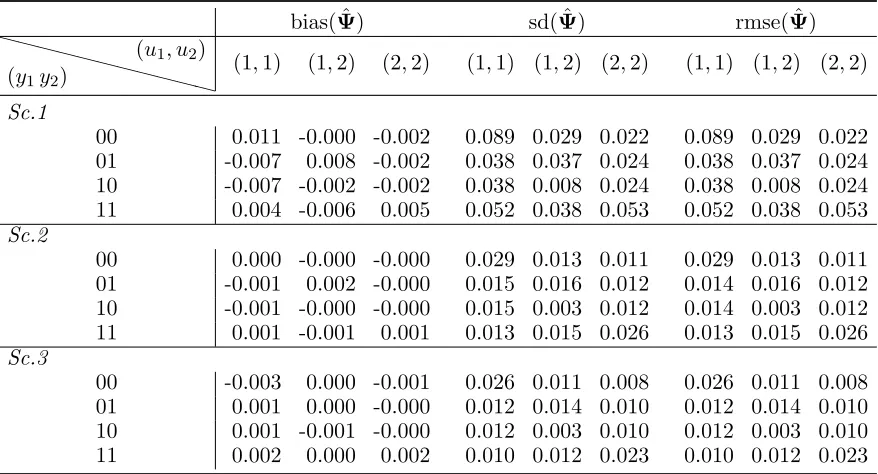
Tables 1-3 report the simulation results for the dynamic SBM with k = 2 hidden states under the different experimental scenarios. The results are based onB = 200 simulated datasets. The performance of our approach is evaluated in terms of bias, standard deviation (sd), and root mean square error (rmse) of the estimators.

By looking at the estimated rmses, we observe that, in general, the quality of the results improves when the number of measurement occasions increases (Scenario 2) and, more

substan-tially, when a higher number of units is available (Scenario 3). Focusing on the parameters of the latent process, it may be noticed that the initial probability vector is estimated with slightly

lower accuracy than the transition matrix, regardless the value ofnand T.

As for the parameters of the latent Markov process, parameters defining the conditional

re-sponse probability of the dyads are estimated with high accuracy, in terms of bias, and precision, in terms of variability; see Table 3. When both the dimension of the network and the number of

observed snapshots increase, the variability of the parameter estimates seems to reduce, ensuring the consistency of the proposed estimation approach in recovering the true data structure.

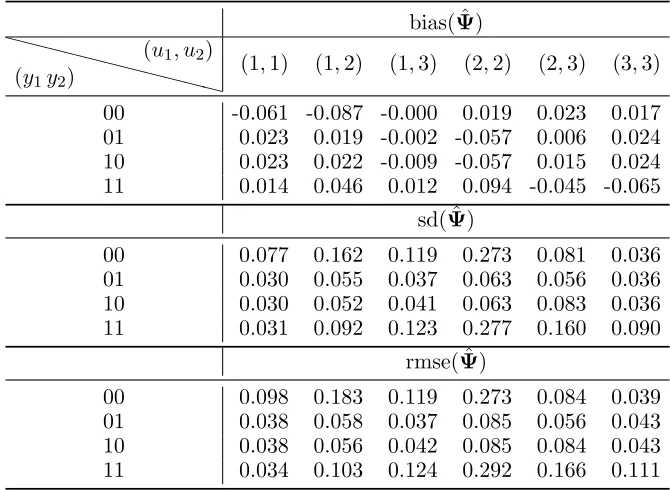
Tables 4-8 report the estimation results for the dynamic SBM withk= 3 latent states under the three experimental scenarios. As expected, the quality of the results obtained under this

model specification turns out to be lower with respect to that observed for the model withk= 2 states due to the higher uncertainty on the latent structure of the model. A higher bias and a

Table 1: Bias, standard deviation (sd), and root mean square error (rmse) for the estimator of the initial probabilities (λu) under different scenarios, with k = 2 latent states (Sc.1: n =

100, T = 10; Sc.2: n= 100, T = 20; Sc.3: n= 200, T = 10).

Sc.1 Sc.2 Sc.3

bias(ˆλ) sd(ˆλ) rmse(ˆλ) bias(ˆλ) sd(ˆλ) rmse(ˆλ) bias(ˆλ) sd(ˆλ) rmse(ˆλ)

u= 1 -0.007 0.080 0.080 -0.002 0.061 0.061 0.001 0.046 0.046

u= 2 0.007 0.080 0.080 0.002 0.061 0.061 -0.001 0.046 0.046

Table 2: Bias, standard deviation (sd), and root mean square error (rmse) for the estimator of the transition probabilities (λu|v) under different scenarios, with k = 2 latent states (Sc.1:

n= 100, T = 10; Sc.2: n= 100, T = 20; Sc.3: n= 200, T = 10).

bias( ˆΛ_{) sd( ˆ}Λ_{) rmse( ˆ}Λ₎

u= 1 u= 2 u= 1 u= 2 u= 1 u= 2

Sc.1 u= 1 0.000 -0.000 0.061 0.061 0.061 0.061

u= 2 0.000 -0.000 0.047 0.047 0.047 0.047

Sc.2 u= 1 -0.003 0.003 0.028 0.028 0.028 0.028

u= 2 0.002 -0.002 0.025 0.025 0.025 0.025

Sc.3 u= 1 -0.001 0.001 0.025 0.025 0.025 0.025

u= 2 0.000 -0.000 0.023 0.023 0.023 0.023

in agreement with the reduced amount of information which is available for each parameter. A

slight reduction in the rmse values is only observed under Scenario 3 due to a higher number of units in the network. When focusing on the estimation of the transition probabilities reported

in Table 5, a higher accuracy and a reduced variability of parameter estimates may be observed, with very few exceptions, which are due to certain samples corresponding to estimates that

considerably differ from those obtained for the other samples.

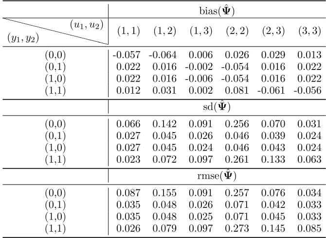
Tables 6-8 report the estimated parameters for the conditional response probabilities of

the dyads under the three experimental scenarios. On the basis of these results, we notice that parameter estimates present quite a similar behaviour with respect to those observed for

the initial and the transition probabilities. The quality of results improves when a higher number of units or a higher number of repeated measurements is available. Thus, based on

Table 3: Bias, standard deviation (sd), and root mean square error (rmse) for the estimator of the conditional response probabilities (ψ_y1y2|u1u2) under different scenarios, withk= 2 latent states (Sc.1: n= 100, T = 10; Sc.2: n= 100, T = 20; Sc.3: n= 200, T = 10).

bias( ˆΨ_{) sd( ˆ}Ψ_{) rmse( ˆ}Ψ₎

❳❳ ❳❳

❳❳ ❳❳

❳❳_❳ (y1y2)

(u1, u2)

(1,1) (1,2) (2,2) (1,1) (1,2) (2,2) (1,1) (1,2) (2,2)

Sc.1

00 0.011 -0.000 -0.002 0.089 0.029 0.022 0.089 0.029 0.022 01 -0.007 0.008 -0.002 0.038 0.037 0.024 0.038 0.037 0.024 10 -0.007 -0.002 -0.002 0.038 0.008 0.024 0.038 0.008 0.024 11 0.004 -0.006 0.005 0.052 0.038 0.053 0.052 0.038 0.053

Sc.2

00 0.000 -0.000 -0.000 0.029 0.013 0.011 0.029 0.013 0.011 01 -0.001 0.002 -0.000 0.015 0.016 0.012 0.014 0.016 0.012 10 -0.001 -0.000 -0.000 0.015 0.003 0.012 0.014 0.003 0.012 11 0.001 -0.001 0.001 0.013 0.015 0.026 0.013 0.015 0.026

Sc.3

00 -0.003 0.000 -0.001 0.026 0.011 0.008 0.026 0.011 0.008 01 0.001 0.000 -0.000 0.012 0.014 0.010 0.012 0.014 0.010 10 0.001 -0.001 -0.000 0.012 0.003 0.010 0.012 0.003 0.010 11 0.002 0.000 0.002 0.010 0.012 0.023 0.010 0.012 0.023

5

Application: Enron email network

A large set of email messages was made public during the legal investigation concerning the Enron corporation. The row Enron corpus (Klimt and Yang, 2004) consists of 619,446 messages

that were sent or received by 158 users between 1998 and 2002; the processed version contains information on 200,399 messages with an average of 757 emails per user. Following Tang et al.

(2008), we first considered only communications recorded between April, 2001 and March, 2002 involving users who sent and received at least 5 emails during that period, thus obtaining a

total number of users equal to 2,359. To further reduce the dimensionality of the network and preserve the real data structure, we randomly chose, among these 2,359 users, n = 151 Enron employees to build up the data matrix. In this application, y(_ijt) = 1 if user i sent at least one email message to user j during the t-th month of the analysed time window, with

i= 1, . . . ,150, j=i+ 1, . . . ,151 and t= 1, . . . ,12.

Here, the interest is in understanding the evolution of dyadic relations between users (email

Table 4: Bias, standard deviation (sd), and root mean square error (rmse) for the estimator of the initial probabilities (λu) under different scenarios, with k = 3 latent states (Sc.1: n =

100, T = 10; Sc.2: n= 100, T = 20; Sc.3: n= 200, T = 10).

Sc.1 Sc.2 Sc.3

bias(ˆλ) sd(ˆλ) rmse(ˆλ) bias(ˆλ) sd(ˆλ) rmse(ˆλ) bias(ˆλ) sd(ˆλ) rmse(ˆλ)

u= 1 0.064 0.147 0.160 0.050 0.152 0.159 0.059 0.128 0.140

u= 2 -0.087 0.202 0.220 -0.101 0.196 0.220 -0.107 0.161 0.193

u= 3 0.023 0.158 0.159 0.051 0.142 0.150 0.048 0.136 0.144

Table 5: Bias, standard deviation (sd), and root mean square error (rmse) for the estimator of the transition probabilities (λ_u|v) under different scenarios, with k = 3 latent states (Sc.1:

n= 100, T = 10; Sc.2: n= 100, T = 20; Sc.3: n= 200, T = 10).

bias( ˆΛ_{) sd( ˆ}Λ_{) rmse( ˆ}Λ₎

u= 1 u= 2 u= 3 u= 1 u= 2 u= 3 u= 1 u= 2 u= 3

Sc.1 u= 1 0.031 -0.044 0.013 0.079 0.098 0.059 0.085 0.108 0.061

u= 2 0.039 -0.071 0.033 0.127 0.173 0.154 0.132 0.187 0.157

u= 3 0.018 -0.048 0.029 0.067 0.092 0.089 0.070 0.104 0.093

Sc.2 u= 1 0.039 -0.063 0.024 0.059 0.077 0.050 0.071 0.100 0.055

u= 2 0.029 -0.031 0.002 0.106 0.127 0.100 0.110 0.130 0.100

u= 3 0.017 -0.055 0.038 0.048 0.070 0.055 0.051 0.089 0.066

Sc.3 u= 1 0.027 -0.048 0.021 0.075 0.083 0.051 0.079 0.095 0.055

u= 2 0.052 -0.079 0.027 0.108 0.147 0.114 0.119 0.166 0.117

u= 3 0.016 -0.059 0.043 0.050 0.075 0.068 0.052 0.095 0.081

Also, in order to reduce the change of being trapped in local maxima, we adopted the multi-start strategy described in Section 3.1; for each value of k = 2, . . . ,6, we retained the best solution according to the CL-BIC and CL-AIC indexes. Results are reported in Table 9.

As it frequently happens, BIC-type indexes are more conservative than the corresponding

AIC ones, suggesting to select a model with a lower number of parameters. In the present framework, CL-BIC leads to selecting a model with k = 3 latent states, while CL-AIC prefers the solution withk= 4 states. In the following, we discuss results for both choices in order to assess the sensitivity of the parameter estimates to the valuek.

5.1 Dynamic SBM with k_{= 3 latent states}

Table 6: Bias, standard deviation (sd), and root mean square error (rmse) for the estimator of the conditional response probabilities (ψ_y1y2|u1u2) under Scenario 1 (n = 100, T = 10), with

k= 3 latent states.

bias( ˆΨ₎

❳❳ ❳❳

❳❳ ❳❳

❳❳_❳ (y1y2)

(u1, u2)

(1,1) (1,2) (1,3) (2,2) (2,3) (3,3) 00 -0.061 -0.087 -0.000 0.019 0.023 0.017 01 0.023 0.019 -0.002 -0.057 0.006 0.024 10 0.023 0.022 -0.009 -0.057 0.015 0.024 11 0.014 0.046 0.012 0.094 -0.045 -0.065

sd( ˆΨ₎

00 0.077 0.162 0.119 0.273 0.081 0.036 01 0.030 0.055 0.037 0.063 0.056 0.036 10 0.030 0.052 0.041 0.063 0.083 0.036 11 0.031 0.092 0.123 0.277 0.160 0.090

rmse( ˆΨ₎

00 0.098 0.183 0.119 0.273 0.084 0.039 01 0.038 0.058 0.037 0.085 0.056 0.043 10 0.038 0.056 0.042 0.085 0.084 0.043 11 0.034 0.103 0.124 0.292 0.166 0.111

combination of latent states keeping in mind the constraints defined in equation (2) and (3). Based on these results, we are able to identify three groups having quite a different profile.

The first hidden state corresponds toinactive users, that is, employees that do not interact with any peers. As suggested by Yang et al. (2011), this represents a necessary state to account for

the sparsity of the data matrix. Hidden states 2 and 3 identify instead active users. More in detail, we may distinguish a group of units (those in state 2) that do not interact with any peers

in the same group (ψ00|22= 1), but that have a quite high chance of receiving emails from units in the third state (ψ_01|23 = 0.51). Also, mutual communications between units in state 3 at a given occasion are highly likely (ψ11|33= 0.85).

The obtained results suggest the presence of three different communication profiles in the Enron

company: inactive (state 1),email receivers (state 2) and email senders (state 3). Clearly, the estimates discussed so far allow us to characterise email exchange between Enron employees

at a given month of the analysed observation window. To understand how the email traffic of the company evolves over time, we may analyse the estimates of parameters defining the

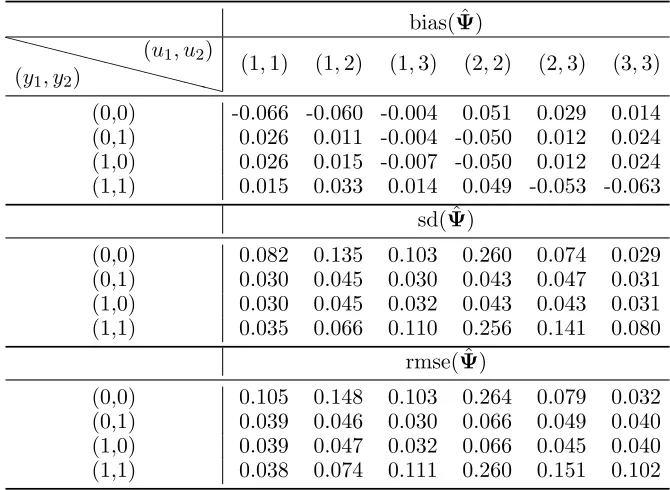
Table 7: Bias, standard deviation (sd), and root mean square error (rmse) for the estimator of the conditional response probabilities (ψ_y1y2|u1u2) under Scenario 2 (n = 100, T = 20), with

k= 3 latent states.

bias( ˆΨ₎

❳❳ ❳❳

❳❳ ❳❳

❳❳_❳ (y1, y2)

(u1, u2)

(1,1) (1,2) (1,3) (2,2) (2,3) (3,3) (0,0) -0.066 -0.060 -0.004 0.051 0.029 0.014 (0,1) 0.026 0.011 -0.004 -0.050 0.012 0.024 (1,0) 0.026 0.015 -0.007 -0.050 0.012 0.024 (1,1) 0.015 0.033 0.014 0.049 -0.053 -0.063

sd( ˆΨ₎

(0,0) 0.082 0.135 0.103 0.260 0.074 0.029 (0,1) 0.030 0.045 0.030 0.043 0.047 0.031 (1,0) 0.030 0.045 0.032 0.043 0.043 0.031 (1,1) 0.035 0.066 0.110 0.256 0.141 0.080

rmse( ˆΨ₎

(0,0) 0.105 0.148 0.103 0.264 0.079 0.032 (0,1) 0.039 0.046 0.030 0.066 0.049 0.040 (1,0) 0.039 0.047 0.032 0.066 0.045 0.040 (1,1) 0.038 0.074 0.111 0.260 0.151 0.102

of the observation period (ˆλ1 = 0.66). Furthermore, state 1 almost represents an absorbing state with a persistence probability equal to ˆλ_1|1 = 0.98. This result can be related to the sparsity of the data matrix observed over all the analysed time window. Concerning the other latent states, persistence over time is quite evident (ˆλ_2|2 = ˆλ_3|3 = 0.84). Some transitions may still be observed, with units in the email receiver group that move with probability ˆλ1|2 = 0.10 towards the inactive state and with probability ˆλ_3|2 = 0.13 towards the email sender group in two subsequent measurement occasions.

5.2 Dynamic SBM with k_{= 4 latent states}

We show in Table 12 the estimated parameters and the corresponding standard errors of the

con-ditional response probabilities under the dynamic SBM withk= 4 latent states. As described in Section 5.1, also in this case, results reported in Table 12 allow us to distinguish betweeninactive

andactive users. The former do not send/receive emails neither from/to employees in the same group, nor from/to employees being in other latent states. On the other hand,active users are classified in three different latent states corresponding to different communication profiles.

Table 8: Bias, standard deviation (sd), and root mean square error (rmse) for the estimator of the conditional response probabilities (ψ_y1y2|u1u2) under Scenario 3 (n = 200, T = 10), with

k= 3 latent states.

bias( ˆΨ₎

❳❳ ❳❳

❳❳ ❳❳

❳❳_❳ (y1, y2)

(u1, u2)

(1,1) (1,2) (1,3) (2,2) (2,3) (3,3) (0,0) -0.057 -0.064 0.006 0.026 0.029 0.013 (0,1) 0.022 0.016 -0.002 -0.054 0.016 0.022 (1,0) 0.022 0.016 -0.006 -0.054 0.016 0.022 (1,1) 0.012 0.031 0.002 0.081 -0.061 -0.056

sd( ˆΨ₎

(0,0) 0.066 0.142 0.091 0.256 0.070 0.031 (0,1) 0.027 0.045 0.026 0.046 0.039 0.024 (1,0) 0.027 0.045 0.024 0.046 0.043 0.024 (1,1) 0.023 0.072 0.097 0.261 0.133 0.063

rmse( ˆΨ₎

(0,0) 0.087 0.155 0.091 0.257 0.076 0.034 (0,1) 0.035 0.048 0.026 0.071 0.042 0.033 (1,0) 0.035 0.048 0.025 0.071 0.045 0.033 (1,1) 0.026 0.079 0.097 0.273 0.145 0.085

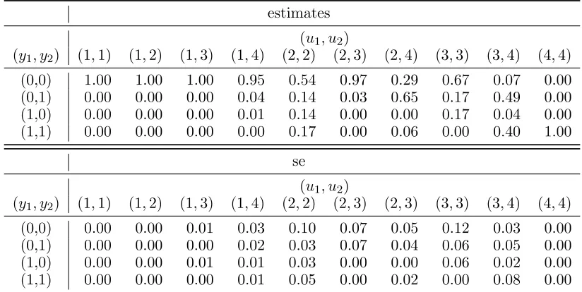
( ˆψ11|44 = 1) and by a high chance of sending email both to units in the second and the third latent state ( ˆψ_01|24 = 0.65,ψˆ_01|34 = 0.49). Such a state can be labelled as the global sender

group. Regarding states 2 and 3, the distinction between them is mainly associated with the observed relations with units in the fourth latent state. State 2 corresponds to receiver only

users ( ˆψ01|24= 0.65), while state 3 identifies employees that are both senders and receivers with respect to the fourth latent group ( ˆψ_01|34 = 0.49,ψˆ_11|34 = 0.40). This state can be labelled as thesender/receiver group.

When analysing the estimated initial and transition probabilities, we get similar results as those

derived for the dynamic SBM withk= 3 latent states; see Table 13. Theinactivelatent states is the most likely one at the beginning of the observation window. Also, the probability of

Table 9: Enron data. CL-BIC and CL-AIC for different choices of k.

latent statesk

2 3 4 5 6

CL-BIC 45857.94 44417.88 _{44428.89 44580.84 44625.63}

Table 10: Enron data. Estimates and estimated standard errors (se) for the conditional response probabilities of the dynamic SBM with k= 3 latent states.

estimates se

(u1, u2)

(y1, y2) (1,1) (1,2) (1,3) (2,2) (2,3) (3,3) (1,1) (1,2) (1,3) (2,2) (2,3) (3,3) (0,0) 1.00 1.00 0.95 1.00 0.33 0.01 0.00 0.00 0.01 0.00 0.03 0.02 (0,1) 0.00 0.00 0.04 0.00 0.51 0.07 0.00 0.00 0.01 0.00 0.02 0.01 (1,0) 0.00 0.00 0.01 0.00 0.04 0.07 0.00 0.00 0.00 0.00 0.00 0.01 (1,1) 0.00 0.00 0.01 0.00 0.11 0.85 0.00 0.00 0.00 0.00 0.02 0.04

Table 11: Enron data. Estimates and estimated standard errors (se) for the latent Markov model parameters of the dynamic SBM withk= 3 latent states.

estimates se

v λˆv λˆ1|v λˆ2|v λˆ3|v λˆv λˆ1|v λˆ2|v λˆ3|v

1 0.66 0.98 0.02 0.00 0.05 0.01 0.01 0.00 2 0.21 0.10 0.84 0.06 0.04 0.03 0.03 0.02 3 0.13 0.03 0.13 0.84 0.03 0.01 0.05 0.05

observing no transitions from this latent state is close to 1 (ˆλ_1|1 = 0.98), thus highlighting the sparsity of the network that remains persistent over all the analysed time window. Similarly, for the other hidden states, transitions are quite unlikely. In particular, units in the receiver only

group tend to move towards the inactive group (ˆλ1|2 = 0.14), while units in the global sender group move towards the sender/receiver one (ˆλ_3|4 = 0.14). Finally, transitions between state 3 and 4 and between state 3 and 2 within two subsequent measurement occasions seems to be almost equally likely (ˆλ_2|3 = 0.10,λˆ_4|3 = 0.12).

6

Concluding remarks

In this paper we discuss dynamic stochastic blockmodels (SBMs) for dynamic networks in a hidden Markov model framework. In this perspective, we are able to identify groups of units

characterised by similar profiles, whose composition may change over time. In order to relax the local independence assumption which is typically used when dealing with dynamic SBMs,

we analyse the dyads referred to ordered pairs of units.

Reciprocal relations between units in the network are described by means of a bivariate latent

Table 12: Enron data. Estimates and estimated standard errors (se) for the conditional response probabilities of the dynamic SBM with k= 4 latent states.

estimates (u1, u2)

(y1, y2) (1,1) (1,2) (1,3) (1,4) (2,2) (2,3) (2,4) (3,3) (3,4) (4,4) (0,0) 1.00 1.00 1.00 0.95 0.54 0.97 0.29 0.67 0.07 0.00 (0,1) 0.00 0.00 0.00 0.04 0.14 0.03 0.65 0.17 0.49 0.00 (1,0) 0.00 0.00 0.00 0.01 0.14 0.00 0.00 0.17 0.04 0.00 (1,1) 0.00 0.00 0.00 0.00 0.17 0.00 0.06 0.00 0.40 1.00

se (u1, u2)

(y1, y2) (1,1) (1,2) (1,3) (1,4) (2,2) (2,3) (2,3) (3,3) (3,4) (4,4) (0,0) 0.00 0.00 0.01 0.03 0.10 0.07 0.05 0.12 0.03 0.00 (0,1) 0.00 0.00 0.00 0.02 0.03 0.07 0.04 0.06 0.05 0.00 (1,0) 0.00 0.00 0.01 0.01 0.03 0.00 0.00 0.06 0.02 0.00 (1,1) 0.00 0.00 0.00 0.01 0.05 0.00 0.02 0.00 0.08 0.00

Table 13: Enron data. Estimates and estimated standard errors (se) for the latent Markov model parameters of the dynamic SBM withk= 4 latent states.

estimates se

v λˆv ˆλ1|v ˆλ2|v ˆλ3|v ˆλ4|v λˆv λˆ1|v λˆ2|v λˆ3|v λˆ4|v

1 0.68 0.98 0.01 0.00 0.00 0.04 0.01 0.01 0.00 0.00 2 0.08 0.14 0.85 0.00 0.00 0.03 0.06 0.06 0.01 0.00 3 0.14 0.00 0.10 0.78 0.12 0.05 0.00 0.04 0.05 0.04 4 0.09 0.06 0.00 0.17 0.77 0.03 0.03 0.00 0.05 0.04

parameter estimates becomes progressively infeasible as the dimension of the network increases.

For this reason, we propose a composite likelihood approach, defined on all possible pairs of observations. When compared to the Bayesian approaches which are typically used with dynamic

SBMs, the composite likelihood method requires a lower computational effort and, also, allows us to avoid the specification of the prior distribution of model parameters that, in some cases,

may severely affect inferential conclusions.

The behaviour of the proposed approach is evaluated by means of a large scale simulation

study and a real data application. Simulation results suggest that the composite likelihood approach allows us to recover the true data structure with high precision, both for the observed

and the latent part of the model. The analysis of the Enron dataset highlights the capability of the dynamic SBMs for dyads in offering a complete and deep description of the relations

An interesting evolution of the proposed approach may be based on adopting marginal

parametrisation for the conditional distribution of each dyad given the underlying Markov chains. This parametrisation is based on two logits for each response variable (marginal with respect

to the other response variable) and the log-odds ratio that measures the conditional association between reciprocal relations given the latent states. In this way, it would be also possible to allow for individual covariates in the analysis and to formulate more parsimonious models in which, for

instance, the level of conditional dependence is constant across latent states. Also, constraints of interest may be formulated on the Markov chain parameters assuming, for instance, that

the initial distribution corresponds to the stationary distribution. In all cases, the composite likelihood inferential approach developed in this paper can be used in these extended versions

of the model.

Acknowledgments

We acknowledge the financial support from award RBFR12SHVV of the Italian Government (FIRB “Mixture and latent variable models for causal inference and analysis of socio-economic

data”, 2012).

References

Akaike, H. (1973). Information theory and an extension of the maximum likelihood principle. In

Second International Symposium on Information Theory, pages 267–281. Akademinai Kiado.

Bartolucci, F. and Farcomeni, A. (2015). Information matrix for hidden markov models with covariates. Statistics and Computing, 25:515–526.

Bartolucci, F., Farcomeni, A., and Pennoni, F. (2013). Latent Markov Models for Longitudinal Data. Chapman & Hall/CRC Statistics in the Social and Behavioral Sciences. Taylor & Francis.

Bartolucci, F. and Lupparelli, M. (2015). Pairwise likelihood inference for nested hidden markov

chain models for multilevel longitudinal data. Journal of the American Statistical Association, pages 00–00.

the statistical analysis of probabilistic functions of Markov chains.The Annals of Mathematical Statistics, 41:164–171.

Cox, D. R. and Reid, N. (2004). A note on pseudolikelihood constructed from marginal densities.

Biometrika, 91:729–737.

Dempster, A. P., Laird, N. M., and Rubin, D. B. (1977). Maximum likelihood from incomplete data via the EM algorithm. Journal of the Royal Statistical Society. Series B. Methodological, 39:1–38.

Diggle, P., Heagerty, P., Liang, K.-Y., and Zeger, S. (2002).Analysis of longitudinal data. Oxford University Press.

Durante, D. and Dunson, D. B. (2014). Nonparametric bayes dynamic modelling of relational

data. Biometrika.

Gao, X. and Song, P. X.-K. (2010). Composite likelihood Bayesian information criteria for model selection in high-dimensional data. Journal of the American Statistical Association, 105:1531–1540.

Godambe, V. P. (1960). An optimum property of regular maximum likelihood estimation. The Annals of Mathematical Statistics, 31:1208–1211.

Goldenberg, A., Zheng, A. X., Fienberg, S. E., and Airoldi, E. M. (2010). A survey of statistical network models. Foundations and TrendsR in Machine Learning, 2:129–233.

Ho, Q., Song, L., and Xing, E. P. (2011). Evolving cluster mixed-membership blockmodel for

time-evolving networks. In International Conference on Artificial Intelligence and Statistics, pages 342–350.

Hoff, P. D. (2011). Hierarchical multilinear models for multiway data. Computational Statistics and Data Analysis, 55:530–543.

Holland, P. and Leinhardt, S. (1976). Local structure in social networks. Sociological Method-ology, 7:1–45.

Klimt, B. and Yang, Y. (2004). The Enron corpus: a new dataset for email classification research.

Lee, N. and Priebe, C. (2011). A latent process model for time series of attributed random

graphs. Statistical inference for stochastic processes, 14:231–253.

Lindsay, B. G. (1988). Composite likelihood methods. Contemporary Mathematics, 80:221–39.

Nowicki, K. and Snijders, T. A. B. (2001). Estimation and prediction for stochastic

blockstruc-tures. Journal of the American Statistical Association, 96:1077–1087.

Robins, G. and Pattison, P. (2001). Random graph models for temporal processes in social networks. Journal of Mathematical Sociology, 25:5–41.

Sarkar, P. and Moore, A. W. (2005). Dynamic social network analysis using latent space models.

ACM SIGKDD Explorations Newsletter, 7:31–40.

Sarkar, P., Siddiqi, S. M., and Gordon, G. J. (2007). A latent space approach to dynamic embedding of co-occurrence data. In International Conference on Artificial Intelligence and Statistics, pages 420–427.

Tang, L., Liu, H., Zhang, J., and Nazeri, Z. (2008). Community evolution in dynamic multi-mode networks. In 14th ACM SIGKDD International Conference on Knowledge Discovery and Data ining, pages 677–685.

Varin, C., Reid, N., and Firth, D. (2011). An overview of composite likelihood methods.Statistica Sinica, 21:5–42.

Varin, C. and Vidoni, P. (2005). A note on composite likelihood inference and model selection.

Biometrika, 92:519–528.

Welch, L. R. (2003). Hidden Markov models and the Baum-Welch algorithm.IEEE Information Theory Society Newsletter, 53:10–13.

Xing, E. P., Fu, W., Song, L., et al. (2010). A state-space mixed membership blockmodel for dynamic network tomography. The Annals of Applied Statistics, 4:535–566.

Xu, K. (2015). Stochastic block transition models for dynamic networks. In18th International Conference on Artificial Intelligence and Statistics, pages 1079–1087.

Yang, T., Chi, Y., Zhu, S., Gong, Y., and Jin, R. (2011). Detecting communities and their

evolutions in dynamic social networks - a bayesian approach. Machine Learning, 82:157–189.