Munich Personal RePEc Archive
One-way and two-way cost allocation in
hub network problems
Bergantiños, Gustavo and Vidal-Puga, Juan
Universidade de Vigo
2 November 2016
One-way and two-way cost allocation in hub
network problems
∗
G. Berganti˜
nos
†1and J. Vidal-Puga
‡11
Departamento de Estat´ıstica e Investigaci´on Operativa,
Universidade de Vigo, Spain
November 2, 2016
Abstract
We study hub problems where a set of nodes send and receive data from each other. In order to reduce costs, the nodes use a network with a given set of hubs. We address the cost sharing aspect by assuming that nodes are only interested in either sending or receiving data, but not both (one-way flow) or that nodes are interested in both sending and receiving data (two-way flow). In both cases, we study the non-emptiness of the core and the Shapley value of the corresponding cost game.
Keywords: hub network, cost allocation, core, Shapley value.
∗This work is partially supported by research grants ECO2014-52616-R from the
Span-ish Ministerio de Econom´ıa y Competitividad, GRC 2015/014 from Xunta de Galicia, and 19320/PI/14 from Fundaci´on S´eneca de la Regi´on de Murcia.
1
Introduction
Hub networks play a fundamental role in modeling telecommunication, trans-portation, and parcel delivery systems. Assume that there are users located at different geographical nodes who need to send a certain flow of data or goods to each other through costly connections. A planner needs to locate an optimal number of hub facilities at some nodes so that each other node is connected to exactly one hub and all the hubs are connected to one another at a reduced cost (due to economies of scale). Hence, the optimal flow of data/goods between any pair of origin-destination nodes has a length of at most four: It must go from the point of origin to its assigned hub (when the origin is not itself a hub), then to the hub assigned to the destination (if it is a different node) and finally to the destination (again, if it is not itself a hub). This topology is applied to Internet connections (Bailey, 1997), telecommu-nications between local networks (Greenfield, 2000), satellite communication (Helme and Magnanti, 1989), airline networks (Bryan and O’Kelly, 1999; Yang, 2009), and small package delivery (Sim et al., 2009).
Several classes of hub problems have been studied. We mention some of them. Aykin (1994) considers that hubs have limited capacities and direct connections between nohubs are allowed. Ernst and Krishnamoorthy (1999) consider the case where there are capacity restrictions but they apply only to the traffic arriving at hubs from nohubs. Sasaki and Fukushima (2003) consider the case where there are capacity constraints on hubs and arcs. Labb´e et al. (2005) consider the case where each hub has a limited capacity as regard the traffic that passes through it. The main issue addressed in these papers is the study of algorithms for computing optimal ways of sending goods between the nodes in such a way that the total cost is minimized. Of course the location of the hubs plays a relevant role in the minimization problem. See Alumur and Kara (2008) and Farahani et al. (2013) for surveys on this literature.
several kinds of problem. We mention some of them: Guardiola et al. (2009) study production-inventory problems where players share production
pro-cesses and warehouse facilities, Berganti˜nos and Kar (2010), Bogomolnaia
and Moulin (2010), Dutta and Mishra (2012) and Trudeau (2012, 2014) con-sider the cost of connecting agents to a source, Moulin (2014) concon-sider users that need to connect a pair of target nodes in a network, and Alcalde-Unzu et al. (2015) consider the cost of cleaning a river. However, few papers have studied this issue in hub problems. We mention three: in all of them the first step is to consider a class of hub problems, the next is to associate a cooperative game with each problem in the class, and the last is to study the core of such problems. If the core is non empty, an allocation in the core could be considered as a nice way of sharing the cost among the agents.
Skorin-Kapov (1998) studies p-hub allocation problems, where p hubs
must be optimally allocated. Several cooperative games are considered de-pending on who the agents are (nodes or pairs of nodes) and what coalitions can do (whether they must use the optimal network for the whole problem or can construct the optimal network of the reduced problem induced by the coalition). The core of such games is studied. Some games have an empty core but others do not. Finally, the nucleolus of such games is considered.
Skorin-Kapov (2001) studies hub-like networks, which involves a p-hub
median problem where direct connection between nodes is possible. More-over, there are savings when the traffic is high. He defines several associated cooperative games where the set of agents are the links. He shows that some of them can have an empty core, in other cases the core is a singleton, and in other cases it has many points.
constructs a network to minimize the total cost associated with hubs in the coalition and communications initiated also by nodes in the coalition. More-over, each coalition simply assumes that the rest of the nodes do not establish any hub nodes and the coalition can determine the routing of all the traffic generated by the other nodes. Given this, they prove that the core could be empty, but they find a sufficient condition for the non-emptiness of the core and propose an allocation in the core when it is non-empty.
Our also focuses on the cost sharing issue. We consider two cases. In the first case (called one-way flow) we assume, as in Skorin-Kapov (1998, 2001) and Matsubayashi et al. (2005), that nodes are only interested in sending flow. In the second case (called two-way flow) we assume that agents are interested in both sending and receiving flow. Internet connections are a good example of situations covered by this case.
We study the existence of core allocations and, unlike Skorin-Kapov (1998, 2001) and Matsubayashi et al. (2005), we also present and charac-terize two rules that belong to the core and also satisfy other nice properties. We now summarize our results for one-way flow. We consider two cooper-ative games associated with each hub problem and related to those presented by Skorin-Kapov (1998). In the first game we assume that nodes can only use the optimal network for the whole problem. In the second game we consider that nodes can construct their own optimal networks. In both games, when we compute the cost of a coalition we consider only the flow sent by nodes in the coalition.
selection (the allocation must be in the core) and equal treatment on hubs (if the cost of a hub increases then any pair of agents such that either both need the hub or neither needs the hub are affected in the same way). The second characterization uses positivity (no node can obtain profits), equal treatment on hubs, independence of irrelevant hubs (nodes are not affected by a change in the cost of hubs that they do not need), and independence of irrelevant flows (if the flow between two nodes increases, other agents should not be affected).
We now summarize our results for the two-way flow. The study is similar to the one-way flow. We associate two games. The first game is concave and hence its core is non empty. It consists of the convex hull of the vector of marginal contributions. The second game could have an empty core.
We study the Shapley value of the first game. Since the game is concave it belongs to the core. We prove that the Shapley value corresponds to the allocation where the cost of sending flow between any pair of nodes is divided equally between the two nodes. Moreover, the cost of each hub is divided equally between the nodes that need the hub to send or receive their flows. Finally, we provide two axiomatic characterizations. The first one uses core selection, equal treatment on hubs, and equal treatment on flows (if there is a flow between a pair of nodes and it increases then both nodes must be affected in the same way). The second characterization uses positivity, independence of irrelevant hubs, independence of irrelevant flows, equal treatment on hubs, and equal treatment on flows.
2
The model
We consider situations where a group of agents, located at different points, want to send and receive some specific good, which is sent through a costly network. Besides, we could locate some hubs in the agent’s points. All hub agents are connected among them but each non-hub agent is connected to only a hub agent. We now introduce the model formally.
N ={1, . . . , n} is a finite set of nodes (also called agents).
C= (cij)i,j∈N is a cost matrix. For eachi, j ∈N, cij is the cost of sending
a unit of flow from node i to node j. We assume cii = 0, cij =cji ≥ 0 and
cik ≤cij +cjk for all i, j, k ∈N.
F = (fij)i,j∈N is the flow matrix. For each i, j ∈ N, fij represents the
amount of flow from node i to node j. We assume fij ≥ 0 and fii = 0 for
all i, j ∈ N. Notice that we do not assume fij = fji, i.e. the flow is not
necessarily symmetric.
d = (di)i∈N indicates the cost of maintaining or constructing a hub at
each node. We assume di ≥0 for all i∈N.
α ∈[0,1] is the discounting factor of the cost when flow goes between a
pair of hubs. Namely, if i and j are both hubs, then the cost of sending a
unit of flow from i to j is αcij (instead of cij)1.
The first issue is to locate an optimal number of hubs, selected from the set of nodes. Besides, each non-hub is linked to exactly one hub and all the hubs are connected to each other. The triangular inequationcik ≤cij+cjk assures
that the optimal path origin-destination uses at most two hubs. When there is a hub in node i∈N, we say with some abuse of notation that node i is a
hub. Otherwise, we say that node i is a non-hub.
A hub network on N is determined by a nonempty set H ⊆ N and a function h:N \H −→H such thath(i) is the hub linked to non-hub i. Let
H be the set of all hub networks onN. For notational convenience, we write
h(i) = i when i ∈ H, so that h is a function from N onto H. Besides, we
1A generalization would be to assume that these costs are given by another cost matrix
Ch= chij
i,j∈N withc h
also write h for the network associated with the function h. Namely
h={{i, h(i)}:i∈N \H}.
Thus, given two nodes i, j ∈ N, flow from node i to node j goes first from
node i to hub h(i), then to hub h(j) and finally to node j (i =h(i) and/or
h(i) = h(j) and/or h(j) = j are possible).
The cost of a hub network h is given by
X
i∈N
X
j∈N
cih(i)+αch(i)h(j)+ch(j)j
fij +
X
i∈H
di.
For simplicity, we denote
λhij = cih(i)+αch(i)h(j)+ch(j)j
fij
so that the cost is
X
i∈N
X
j∈N
λhij+X
i∈H
di.
A hub networkh∈ H where
min
h∈H
(
X
i∈N
X
j∈N
λhij +X
i∈H
di
)
is reached is called optimal. Since H is finite, there is always at least one optimal hub network.
A hub network problem is a tuple P = (N, C, F, d, α, h) where h is a hub network.
Notice that we have not assumed that h is an optimal hub network. We
know that to compute an optimal hub network is N P hard. Thus, in many
practical situations we use heuristics to decide the hub network h to be
constructed. Hence, we do not know exactly if such hub network is optimal
or not. We make a very weak assumption on h, all hubs are needed in order
to send the flow. Namely, for all k ∈ H there exist i, j ∈ N with fij > 0
in which some hubs are not needed, in order to make easier the reading, we have decided to present it making this assumption.
We now define c(P) as the cost associated with the hub network h.
Namely,
c(P) = X
i∈N
X
j∈N
λhij +X
i∈H
di. (1)
In many cases after finding an optimal (or quasi optimal) hub network, we need to divide the cost of such network among the agents. Arule is a function
R that assigns to each hub network problem P an allocation R(P) ∈ RN
satisfying
X
i∈N
Ri(P) =c(P). (2)
Our aim is to study the cost allocation problem generated by each hub
network problem P. We are interested into studying fair allocations. The
idea is to propose desirable properties and try to find a rule satisfying many of them.
We consider two cases depending on the needs of the agents. In the
one-way flow case, we assume that each agent is only interested in the flow that leaves from it (the case where each agent is only interested in the flow that arrives to it is similar). In the two-way flow case, each agent is interested in both the flow that arrives to it and the flow that leaves from it.
Acost game is a pair (N,ˆc) where N is the set of agents and ˆc: 2N →R
is a cost function satisfying ˆc(∅) = 0. Each nonempty subsetS ⊆N is called a coalition, and ˆc(S) denotes the cost of providing the needs of all agents in
S. Since ˆcdepends on N, we write ˆcinstead of (N,cˆ).
We say that ˆc is concave if for all l ∈ T ⊂ S ⊆ N, we have ˆc(S)−
ˆ
c(S\ {l})≤ˆc(T)−ˆc(T \ {l}).
The core of a cost game ˆc is defined as
Core(ˆc) = (
y∈RN :X
i∈N
yi = ˆc(N) and
X
i∈S
yi ≤ˆc(S)∀S⊂N
)
.
The Shapley value (Shapley, 1953) is defined as the allocationSh(ˆc) such that
Shi(ˆc) =
X
S⊂N\{i}
|S|! (n− |S| −1)!
n! [ˆc(S∪ {i})−ˆc(S)]
for each i∈N.
3
One-way flow
In this section, we assume that agents are interested only in the flow that leaves. The case in which they are interested only in the flow that arrives is completely analogous. We first associate to each hub network problem a cost game. Later we study the core and the Shapley value of such game.
For each hub network problem P, we associate the cost game cofP where
for each S ⊆N, cofP (S) is the cost of sending the flow of all agents in S to all agents through the hub network h. The cost game cofP models situations
where the hub network h (with associated set of hubs H) has already been
constructed. Thus, d could be considered as a vector of maintenance costs.
Agents in each coalition are only interested in the hubs they need for sending their flow. We now define this cost game formally.
For each S ⊆N, let HSof ⊆H denote the set of hubs needed for sending the flow of agents in S. Namely,
HSof ={k ∈H :∃i∈S, j ∈N with fij >0 and k ∈ {h(i), h(j)}}.
Given i∈N, we writeHiof instead ofH{i}of. Notice that HSof =S
i∈SH of i
for all S⊆N. Now,
cofP (S) = X
i∈S
X
j∈N
λhij+ X
i∈HSof
di. (3)
When no confusion arises we write cof(S) instead of cof P (S).
be considered as a generalization of c1. In our model when h has p hubs and
di = 0 for all i, cofP coincides with c1. Besides, Skorin-Kapov (1998) proves
that the core of c1 contains the single allocation where each agents pays the cost of sending its flow.
3.1
The core
In the next theorem we prove that the core of cof is the set of allocations in
which each agent pays the cost of sending its flow. Besides, the cost of any hub is divided in any way among the agents that need the hub for sending its flow.
Theorem 3.1 For each hub network problem P the core of cof is nonempty,
and it is given by
Core cof =
(
x∈RN :P
i∈Nxi =c(P), xi =
P
j∈Nλhij +yi∀i∈N
where y ∈RN
+ and
P
i∈Syi ≤
P
i∈HofS di∀S ⊂N
)
.
Proof. “⊇” is obvious.
We now prove “⊆”. Let x ∈ Core cof
. Then, for each i ∈ N, xi =
P
j∈Nλhij +yi where yi = xi −
P
j∈Nλhij. Since, x ∈ Core cof
, for each
S ⊂N,
cof(S) = X
i∈S
X
j∈N
λhij + X
i∈HSof
di ≥
X
i∈S
xi =
X
i∈S
X
j∈N
λhijN +X
i∈S
yi
and thus P
i∈Syi ≤ Pi∈Hof
S di. It only remains to prove that y ∈ R
N
+.
Suppose not. Let j ∈N be such thatyj <0. Thus,
X
i∈N\{j}
xi =
X
i∈N
xi−xj =cof(N)−xj
=X
i∈N
X
j∈N
λhij +X
i∈H
di−
X
j∈N
λhij −yj
= X
i∈N\{j}
X
j∈N
λhij +
X
i∈H
di −yj
> X
i∈N\{j}
X
j∈N
λhij +X
i∈H
since HN\{j}of ⊆H,
> X
i∈N\{j}
X
j∈N
λhijN + X
i∈HNof\{j}
di =cof(N \ {j})
which is a contradiction.
Skorin-Kapov (1998) also considers the game c∗
1, which is obtained asc1
but assuming that each coalition can build their optimal network. Namely,
instead of using the hubs given by h, each coalition can locate hubs where
they want. Skorin-Kapov (1998) proves that the core of c∗
1 could be empty.
In our case the same happens. The core ofcof∗ could be empty. We will
see it by proving that the core of the following intermediate situation could be also empty.
Assume that the optimal hub network is not unique. Thus, we should decide which one to construct. It could be the case that some agents prefer one over the other (for instance if an agent is a hub the cost of sending their flow should be smaller). Thus, we can define the cost of a coalition as the
minimum over all optimal hub networks. Namely, for each S⊆N,
c∗(S) = min
h∈H,his optimal
n
cofP(h)(S)o
whereP(h) is the hub network problem induced by the optimal hub network
h. Next example shows that the core of c∗ can be empty.
Example 3.1 LetN ={1,2,3}, cij = 1for alli, j ∈N,f12 =f23 =f31= 1,
f21 = f32 = f13 = 10, α = 1, and di = 6 for all i ∈ N. There exist three
optimal hub networks {hi}
i∈N, corresponding to putting a single hub in each
node i∈N, respectively. Furthermore, each two-node coalition would prefer a different hub location. Coalition {1,2} would prefer the hub to be at 1, because
cofP(h1
)({1,2}) = 29≤min
n
cofP(h2
)({1,2}), c
of P(h3
)({1,2})
o ;
coalition {1,3} would prefer to locate the hub at 3, because
cofP(h3)({1,3}) = 29≤min
n
cofP(h1)({1,3}), c
of
P(h2)({1,3})
and coalition {2,3} would prefer to locate the hub at 2, because
cofP(h2)({2,3}) = 29≤min
n
cofP(h1)({2,3}), c
of
P(h3)({2,3})
o
.
Let x be a core allocation. Then
100 = 2c∗(N) = 2 (x1+x2+x3)
= (x1 +x2) + (x1 +x3) + (x2+x3)
≤cofP(h1
)({1,2}) +c
of P(h3
)({1,3}) +c
of P(h2
)({2,3})
= 29 + 29 + 29 = 87,
which is a contradiction.
Thus, the core of c∗ is empty.
3.2
The Shapley value
We now study the Shapley value of cof, which we call the Shapley rule. We
first give an explicit formula. Later, we provide two axiomatic characteriza-tions.
In the next theorem we prove that in the Shapley rule each agent pays the cost of sending its flow. Besides, the cost of any hub is divided equally among the agents that need the hub for sending their flow.
Theorem 3.2 For each hub network problem P and each i∈N,
Shi
cofP =X
j∈N
λhij + X
j∈Hofi
dj
n
k ∈N :j ∈Hkofo
.
Proof. We consider several cost games. Let c0 be defined as c0(S) =
P
i∈S
P
j∈Nλhij for eachS ⊆N. For eachj ∈N, letcj be defined ascj(S) =
dj if j ∈ HSof and cj(S) = 0 otherwise. Thus, for each S ⊆ N, cof(S) =
c0(S) +P
j∈N cj(S). Since the Shapley value is additive on c, we have that
for each i∈N, Shi cof
game (there exists a ∈RN such that for each S ⊆ N, c0(S) = P
j∈Sai) we
deduce that Shi(c0) = Pj∈Nλhij. For each j ∈ N, in the cost game cj, all
agents that need hub j (i.e. all k∈N such thatj ∈Hkof) are symmetric and
the agents that do not need hub j are dummy. Thus, for each j ∈N,
Shi cj
=
dj
|{k∈N:j∈Hkof}| if j ∈H of i
0 otherwise,
from where it is straightforward to check the result. We now define several properties.
The first property says that no agent should obtain profit.
Positivity (P os) For any hub network problem P and eachi∈N, we have
Ri(P)≥0.
The second property says that equal agents must pay the same. Consider the following example.
Example 3.2 Let P be such that N ={1,2,3}, cij = 3 and fij = 1 for all
i, j ∈ N,and di = 6 for all i ∈ N. There are three optimal hub networks.
We construct a hub in node i and we join the other nodes to node i. Thus,
c(P) = 30. Assume that h is the optimal hub network where the hub is at
node 1 (the other cases are analogous). Thus,cof is defined as follows:
S {1} {2} {3} {1,2} {1,3} {2,3} {1,2,3}
cof (S) 12 15 15 21 21 24 30.
Notice that even agents are symmetric in C, F, and d. Nevertheless, in cof,
agents 2 and 3 are symmetric but agents 1 and 2 are not.
Since we are dealing with situations whereh is given, we should consider such hub network when defining equal nodes. Thus, given a hub network
problem P we say that nodesiandj areequal when several conditions hold:
First, fik =fjk for all k ∈N \ {i, j}. Second,fij =fji. Third, i∈ H if and
{i, k} ∈ h if and only if {j, k} ∈ h (namely, if nodes i and j are nonhubs then both are connected to the same hub). Fifth, for each {i, k},{j, k} ∈h,
cik =cjk.
Equal Treatment of Equals (ET E) For any hub network problemP and each pair of equal nodes i, j ∈N, we have that Ri(P) =Rj(P).
As in the case ofET E, the next properties are defined considering the hub network h as fixed. The first of them says that we must select an allocation in the core of the problem.
Core Selection (CS) For any hub network problem P, we have that
R(P)∈CorecofP .
The next property says that if a node does not send any flow, then it pays nothing.
Null Flow (N F) For any hub network problem P and each i ∈ N such that fij = 0 for allj ∈N \ {i}, we have that Ri(P) = 0.
The next property says that if the flow leaving node i increases, then
node i cannot pay less.
Flow Monotonicity (F M) For any pair of hub network problems P = (N, C, F, d, α, h) andP′ = (N, C, F′, d, α, h) such that there existi, j ∈
N satisfying fij ≥fij′ and fkl =fkl′ otherwise, then Ri(P)≥Ri(P′).
The next property says that if the maintenance cost of a hub increases, then no node requiring such hub could pay less.
Hub Monotonicity (HM) For any pair of hub network problems P = (N, C, F, d, α, h) and P′ = (N, C, F, d′, α, h) such that there exists k ∈
N satisfying dk ≥d′k and dj =d′j otherwise, then for each agent isuch
The next property says that if the cost of a link increases, then the two agents located at its vertices could not pay less.
Cost Monotonicity (CM) For any pair of hub network problems P = (N, C, F, d, α, h) andP′ = (N, C′, F, d, α, h) such that there existsi, j ∈
N satisfying cij ≥ c′ij and ckl = c′kl otherwise, then we have that
Ri(P)≥Ri(P′) and Rj(P)≥Rj(P′).
Assume that the cost of some hub dk decreases. It is then clear that if h
was an optimal hub network in the original problem it will be also optimal in the new problem. How agents should be affected? The next two properties give an answer to this question.
The first one says that agents that need hubk or do not need hub k are
affected in the same way.
Equal Treatment on Hubs (ET H) For any pair of hub network prob-lems P = (N, C, F, d, α, h) and P′ = (N, C, F, d′, α, h) such that there
existsk ∈N satisfying dk ≥d′k and dj =d′j otherwise, then for all pair
of agents i, j such that k∈Hiof ∩Hjof ork /∈Hiof ∪Hjof, we have that
Ri(P)−Ri(P′) =Rj(P)−Rj(P′).
The second one says that agents that do not need hubk are not affected.
Independence of Irrelevant Hubs (IIH) For any pair of hub network problems P = (N, C, F, d, α, h) and P′ = (N, C, F, d′, α, h) such that
there exists k ∈ N satisfying dk ≥ d′k and dj =d′j otherwise, then we
have that Ri(P) =Ri(P′) for each agent i such thatk /∈Hiof.
We now introduce a similar property to IIH but with flows instead of
Independence of Irrelevant Flows (IIF) For any pair of hub network problems P = (N, C, F, d, α, h) and P′ = (N, C, F′, d, α, h) such that
there exist j, k ∈N satisfying 0< f′
jk ≤fjk andfj′′k′ =fj′k′ otherwise,
then we have that Ri(P) =Ri(P′) for each agent i∈N \ {j}.
There are some relations between these properties,
Proposition 3.1 (a) CS implies P os.
(b) P os, IIH and IIF imply CS.
Proof. (a) Assumex∈Core cof
. Then, for all i∈N,
xi =cof(N)−
X
j∈N\{i}
xj ≥cof(N)−cof(N \ {i})≥
X
j∈N\{i}
λhij ≥0.
(b) LetR be a rule satisfying P os, IIH, andIIF. FixS ⊂N. Let ε >0 and define PS,ε = N, C, FS,ε, dS, α, h
as the problem obtained from P by
turning all positive flows not used by S into ε and all hub costs not used by
S into zero. Formally,
fijS,ε= (
ε if i /∈S and fij >0
fij otherwise
and
dSk = (
0 if k /∈HSof dk otherwise.
Then, cofPS,ε(N)≤
P
i∈S
P
j∈Nλhij +
P
k∈HSof dk+a(P)ε where
a(P) = |{fij :fij >0}|max
(
λh ij
fij
:fij >0
)
.
Now,
X
i∈S
Ri(P)
IIH+IIF
= X
i∈S
Ri PS,ε
=cofPS,ε(N)−
X
i∈N\S
Ri PS,ε
P os
≤ cofPS,ε(N)≤
X
i∈S
X
j∈N
λhij + X
k∈HSof
dk+a(P)ε
which implies P
i∈SRi(P)≤cPof(S) because a(P) does not depend on ε.
CS does not imply neither IIH nor IIF. The rule in which each agent
pays the cost of sending its flow and the cost of each hub is paid equally by the agents that use the most expensive hubs among those that use that
hub satisfies CS but not IIH. The rule in which each agent pays the cost
of sending its flow and the cost of each hub is paid equally by the agents
sending more flow through this hub satisfies CS but notIIF.
In the next proposition we prove that the Shapley rule satisfy all the above properties.
Proposition 3.2 The Shapley rule satisfies P os, ET E, CS, N F, F M,
HM, CM, ET H, IIH and IIF.
Proof. From Theorem 3.2, we deduce thatSh cof
satisfiesP os,F M,HM, and CM. If i and j are equal in P, then it is easy to see that i and j are symmetric in cof. Now, symmetry of the Shapley value implies thatSh cof satisfies ET E. Any i∈N with fij = 0 for all j ∈N\ {i}is a dummy player
in cof. Hence, its Shapley value is zero, and so Sh cof
satisfies N F. Let
P, P′ and k be given as in the definition of ET H and IIH. Given i, j ∈ N
such that k ∈Hiof ∩Hjof, by Theorem 3.2
Shi
cofP −Shi
cofP′
= dk−d
′ k
n
l ∈N :k ∈Hlofo
=Shj
cofP −Shj
cofP′
Given i, j ∈N such that k /∈Hiof ∪Hjof, by Theorem 3.2
Shi
cofP −Shi
cofP′
= 0 =Shj
cofP −Shj
cofP′
.
Hence Sh cof
satisfies ET H. Given i∈ N such that k /∈Hiof, from Theo-rem 3.2 we know that Shi cof
does not depend on dk, and so Shi
cofP =
Shi
cofP′
and hence Sh cof
satisfies IIH. Let P, P′ and i, j, k be given as in the definition of IIF. From Theorem 3.2 we have that Shi cof
does not depend on fjk. Hence, Sh cof
satisfies IIF. From Proposition 3.1, it satisfies CS.
Theorem 3.3 (a) The Shapley rule is the unique rule satisfying CS and
ET H.
(b) The Shapley rule is the unique rule satisfying P os, IIH, IIF, and
ET H.
Proof. (a) By Proposition 3.2 the Shapley rule satisfies these properties.
We now prove the uniqueness. Let R be a rule satisfying CS and ET H.
LetP = (N, C, F, d, α, h) be any hub network problem. For eachK ⊆H, let PK = N, C, F, dK, α, h
with dK defined as follows:
dKi = (
0 if i∈H\K
di otherwise.
For all k ∈ N, let Nk,0 = ni∈N :k /∈Hof i
o
, Nk,1 = ni∈N :k ∈Hof i
o ,
nk,0 = Nk,0
and nk,1 = Nk,1
for all k∈N.
ET H implies that, for eachk ∈K, there existxk,0 andxk,1 such that for
all i∈Nk,0,
Ri PK
−Ri PK\{k}
=xk,0 (4)
and for all i∈Nk,1
Ri PK
−Ri PK\{k}
=xk,1. (5)
Since N =Nk,0 ∪Nk,1 and
X
i∈N
Ri PK
−X
i∈N
Ri PK\{k}
=dk
we have that for all k ∈K,
nk,0xk,0+nk,1xk,1 =dk. (6)
The equivalence relation inN defined as
i∼j ⇔ ∃k ∈K :i, j ∈Nk,1 or i, j ∈Nk,0
determines a partition PK of N. It is straightforward to check that the
cost game cofPK(N) =
P
S∈PK c
of
PK(N). So CS implies that
P
i∈SRi PK
cofPK(S) for allS ∈ PK. Moreover, anyPLwith L⊂K is a refinement ofPK,
so P
i∈SRi PL
=cofPL(S) for all S ∈ PK.
We now consider several cases.
Case 1. Assume that PK has at least two components. Given k ∈ K,
there exist S, S′ ∈ P
K such that k ∈ S ∩ H and S′ ⊆ Nk,0. Besides,
cofPK\{k}(S
′) = cof
PK(S′). Thus,
cofPK (S
′
) = X
i∈S′
Ri PK
(4)
= X
i∈S′
Ri PK\{k}
+|S′|xk,0
CS
= cofPK\{k}(S
′) +|S′|xk,0 =cof PK (S
′) +|S′|xk,0
which implies that xk,0 = 0.
By (6),xk,1 = dk
nk,1 for all k∈K. By (5), for eachi∈N,
Ri PK
=Ri PK\{k}
+ dk
nk,1.
Repeating the same argument, we deduce that for each i∈N,
Ri PK
=Ri P∅
+ X
k∈Hiof
dk
nk,1.
SinceR satisfiesCS, under Theorem 3.1,Ri P∅
=P
j∈Nλhij+yi for all
i∈N, where 0≤yi ≤Pj∈Hof i d
∅
j. By definition of d∅, we have d∅j = 0 for all
j ∈H. Since Hiof ⊆H, we deduce yi = 0 and so
Ri P∅
=X
j∈N
λhij.
By Theorem 3.2,
Ri PK
=X
j∈N
λhij + X
k∈Hiof
dk
nk,1 =Shi P
K
.
Case 2. Assume now PK ={N}. We consider several cases.
Case 2.1. Assume K ={k}. Since R satisfies CS, under Theorem 3.1,
X
i∈Nk,0
Ri P{k}
= X
i∈Nk,0
X
j∈N
λhij + X
j∈Nk,0
where y∈RN
+ and
0≤ X
i∈Nk,0
yi ≤
X
j∈Hof
N k,0
d{k}j = 0
which implies P
i∈Nk,0yi = 0. Thus,
X
i∈Nk,0
Ri P{k}
= X
i∈Nk,0
X
j∈N
λhij.
On the other hand,
X
i∈Nk,0
Ri P{k}
(4)
= X
i∈Nk,0
Ri P∅
+nk,0xk,0 = X
i∈Nk,0
X
j∈N
λhij +nk,0xk,0
which implies xk,0 = 0. So, for eachi∈Nk,0,
Ri P{k}
=X
j∈N
λhij =Shi P{k}
.
Under (6), xk,1 = dk
nk,1. So, for each i∈Nk,1,
Ri P{k}
=Ri P∅
+ dk
nk,1 =
X
j∈N
λhij + dk
nk,1 =Shi P
{k}
.
Case 2.2. Assume now |K|>1. We proceed by induction on|K|. Hence,
we assume R PK′
=Sh PK′
when |K′|<|K|. We have three cases:
Case 2.2.1. Assume first nk,0 = 0 for some k ∈ K. By (5), for all i∈N =Nk,1,
Ri PK
=Ri PK\{k}
+xk,1.
Hence,
X
i∈N
Ri PK
=X
i∈N
Ri PK\{k}
+nxk,1
and thus
xk,1 = P
i∈NRi PK
−P
i∈NRi PK\{k}
n =
dk
nk,1.
Now for all i∈N =Nk,1,
Ri PK
=Ri PK\{k}
+ dk
By induction hypothesis, for all i∈N
Ri PK
=X
j∈N
λhij + X
j∈Hiof
dK\{k}j nk,1 +
dk
nk,1
=X
j∈N
λhij + X
j∈Hiof
dK j
nk,1 =Shi P
K
.
Case 2.2.2. Assume now nk,1 = 0 for some k ∈ K. By (4), R
i PK
=
Ri PK\{k}
+xk,0 for all i ∈ N = Nk,0. The rest of reasoning is analogous
to the previous case and we omit it.
Case 2.2.3. Finally, assume nk,0 >0 and nk,1 >0 for all k ∈K. We can
assume w.l.o.g. 1,2 ∈ K. Let i1 ∈ N1,1 and i2 ∈ N1,0. Since P
K = {N},
we know that there exists some k ∈ K such that either i1, i2 ∈ Nk,1 or
i1, i2 ∈ Nk,0. Assume w.l.o.g. that either i1, i2 ∈ N2,1 or i1, i2 ∈ N2,0. For
each k ∈ {1,2} and each l ∈ {1,2}, let fl(k) ∈ {0,1} be defined such that
il ∈ Nk,fl(k)
. Hence, we know that f1(1) = 1 (because i1 ∈ N1,1), f2(1) = 0
(because i2 ∈ N1,0), and f1(2) = f2(2) (because either i1, i2 ∈ N2,1 or i1, i2 ∈N2,0).
By induction hypothesis, for any k∈ {1,2} and any l∈ {1,2},
Ril PK
(4)(5)
= Ril PK\{k}
+xk,fl(k) =Shil PK\{k}
+xk,fl(k)
=X
j∈N
λhil j +
X
j∈Hof
il
dK\{k}j nj,1 +x
k,fl(k)
.
Thus, for eachl ∈ {1,2},
x1,fl(1)−x2,fl(2) = X
j∈Hof
il
dK\{j 1}−dK\{j 2} nj,1 =
d1 n1,1f
l(1)− d2
n2,1f
l(2).
In particular, taking a=f1(2) =f2(2) andl = 1,
x1,1−x2,a = d1
n1,1 − d2
n2,1a (7)
and taking l= 2,
x1,0−x2,a =− d2
Equations (6) fork = 1,2 and equations (7)-(8) can be written as a matrix equation as follows:
n1,1 0 n1,0 0
0 n2,1 0 n2,0
1 −a 0 a−1
0 −a 1 a−1
·
x1,1 x2,1 x1,0 x2,0
= d1 d2 d1
n1,1 − d 2
n2,1a
− d2
n2,1a
.
The determinant of the left matrix is (an−n2,1)n 6= 0. Hence, the matrix
equation has a unique solution given by xk,1 = dk
nk,1 and xk,0 = 0 for all
k ∈ {1,2}. Thus,
Ri1 PK
(5)
= Ri1 PK\{1}
+x1,1 =R
i1 PK\{1}
+ d1
n1,1 Ri2 PK
(4)
= Ri2 PK\{1}
+x1,0 =Ri2 PK\{1}
.
By induction hypothesis,
Ri1 PK
=Shi1 PK\{1}
+ d1
n1,1
T h.3.2
= X
j∈N
λhi1j +
X
k∈Hof
i1
dK\{k 1} nk,1 +
d1 n1,1
=X
j∈N
λhi1j +
X
k∈Hof
i1
dK k
nk,1
T h.3.2
= Shi1 PK
Ri2 PK
=Shi2 PK\{1}
T h.3.2
= X
j∈N
λhi2
j +
X
k∈Hof
i2
dK\{k 1} nk,1
=X
j∈N
λhi2
j + X k∈Hof i2 dK k
nk,1
T h.3.2
= Shi2 PK
.
Since i1, i2 were taken arbitrarily from N1,1 and N1,0, respectively, and
these two sets form a partition of N, we conclude thatRi PK
=Shi PK
for all i∈N.
(b) It follows from part (a) and Proposition 3.1.
• Let R0 be defined as R0(P) = x+Sh cof
for some x ∈ RN with
P
i∈Nxi = 0 and xi 6= 0 for some i ∈ N. R0 satisfies IIH, IIF and
ET H, but fails CS and P os.
• Let ω ∈ RN be such that ωi > 0 for all i ∈ N and ωi 6= ωj for some
i6=j. Let R1 be defined for each P and each i∈N as follows:
R1i (P) = X
j∈N
λhij + X
j∈Hiof
ωi
P
k∈N:j∈Hkof ωk
dj.
R1 satisfies CS, P os, IIH, and IIF, but failsET H.
• Let R2 be defined for each P and i∈N as follows:
Ri2(P) = X
j∈N
λhij +X
j∈H
dj
n.
R2 satisfies P os, IIF and ET H, but fails CS and IIH.
• Let R3 be defined for each P and i∈N as follows:
R3i (P) = P
k∈N
P
j∈Nλhkj
n +
X
j∈Hiof
dj
n
k ∈N :j ∈Hkofo
.
R3 satisfies P os, IIH and ET H,but fails CS and IIF.
4
Two-way flow
In this section we consider the case in which the users are interested in both receiving and sending data. Again, we assume that communication is carried over a (maybe optimal) hub network. We first associate to each hub network problem a cooperative game. Later on we study the core and the Shapley value.
For each hub network problem P we associate the cost game ctfh where
for each S ⊆ N, ctfh (S) is the cost of sending and receiving the flow of all
situations where an (optimal) hub network h (with associated set of hubs
H) has already been constructed. Thus, dcould be considered as a vector of maintenance costs. Agents in each coalition are interested in the hubs they need for sending or receiving their flow. Notice that we are applying the same ideas than in the one-way flow. We now define this cost game formally. For each S ⊆ N, letHStf ⊆ H denote the set of hubs needed for sending or receiving the flow of agents in S. Namely,
HStf =HSof ∪ {k ∈H :∃i∈S, j ∈N with fji >0 andk ∈ {h(i), h(j)}}.
Given i∈N, we write Hitf instead of H{i}tf. Like in the previous section,
HStf =S
i∈SH tf
i for all S ⊆N.
Now,
ctfP(S) = X
(i,j)∈/(N\S)×(N\S)
λhij + X
i∈HStf
di. (9)
When no confusion arises we write ctf instead ofctf P.
4.1
The core
In the next theorem we prove that in the core allocations of ctf the cost
of sending or receiving flow between two nodes is divided between them. Besides, the cost of any hub is divided among the agents that need the hub for sending or receiving their flow. Before stating the theorem we need some notation.
Let Π ={π :N −→N :π biyective} be the set of orderings of agents in
N.
Given i∈N and j ∈H, Πij ⊂Π is the set of orderings such that node i
is the first that uses hub j, i.e. π(l) =i implies j /∈Hπtf(l′) for all l′ < l.
Theorem 4.1 For each hub network problem, ctf is concave. Moreover, the
core is nonempty and given by the convex hull of the following set of vectors:
X
j∈N:π−1(j)>π−1(i)
λhij +λhji
+ X
j∈Hitf:π∈Πij
dj
i∈N
Proof. We first prove that N, ctf
is concave. Let l∈T ⊂S ⊆N.
Since for each S′ ⊂N,Htf S′ =
S
i∈S′Hitf, we have that
HStf\HS\{l}tf ⊂HTtf \HTtf\{l}. (10) Then,
ctf(S′)−ctf(S′ \ {l}) = X
(i,j)∈/(N\S′)×(N\S′)
λhij + X
i∈HS′
di
− X
(i,j)∈/(N\(S′\{l}))×(N\(S′\{l}))
λhij −
X
i∈HStf′\{l}
di
= X
i∈N\S′
λhil+ X
j∈N\S′
λhlj + X
i∈HStf′\HtfS\{l}
di.
Since all terms are non-negative, N \S ⊂N \T and (10), we have that
ctf(S)−ctf(S\ {l})≤ctf(T)−ctf(T \ {l}) which proves that N, ctf
is concave.
It is well known that when the cost game is concave, the core coincides with the Weber set. So it is the convex hull of the vectors of marginal contri-butions. Notice that the coordinatei of the vector of marginal contributions for π ∈Π is
X
j∈N:π−1(j)>π−1(i)
λhij +λhji
+ X
j∈Hitf:π∈Πij
dj,
hence the result holds.
Analogously to the one-way case, we consider now an intermediate situa-tion between a fixed hub network and a variable hub network. Assume that the optimal hub network is not unique and the planner should decide which one to construct. We can define the cost of a coalition as the minimum over
all optimal hub networks. Namely, for each S ⊆N,
c∗∗(S) = min
h∈H,his optimal
n
ctfP(h)(S)o
whereP(h) is the hub network problem induced by the optimal hub network
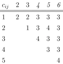
Example 4.1 Let P be such that N = {1,2, . . . ,6}, α = 1, f12 = f34 =
f56 = 1, fij = 0 otherwise. d1 =d2 =d3 = 1and di ≥4 otherwise. The cost
matrix is given in the following table:
cij 2 3 4 5 6
1 2 2 3 3 3
2 1 3 4 3
3 4 3 3
4 3 3
5 4
This hub problem is depicted in Figure 1.
1
2
3
4
5 6
2 1
2
4
[image:27.595.243.353.193.304.2]4 4
Figure 1: cij = 3 when no specified. Flow goes from 1 to 2, from 3 to 4, and
from 5 to 6.
There exist three optimal hub networks {hi}3
i=1, corresponding to putting
a single hub at either 1, 2or 3, respectively. The cost of these networks is 14
each. Hence,c∗∗(N) = 14. Moreover, nodes1,2,3,4can cover their own flow at cost7when the hub is located at2. Then,c∗∗({1,2,3,4}) = 7. Analogously, nodes 1,2,5,6 can cover their own flow at cost 9 when the hub is located at
1, so that c∗∗({1,2,5,6}) = 9. Analogously, nodes 3,4,5,6 can cover their
own flow at cost11when the hub is located at 3, so thatc∗∗({3,4,5,6}) = 11.
Hence, a core allocationyshould satisfyy1+y2+y3+y4 ≤7, y1+y2+y5+y6 ≤
9, and y3+y4+y5+y6 ≤11. By adding these inequalities and dividing by 2, we deduce that P
i∈Nyi ≤13.5. Since c∗∗(N) = 14, we deduce that the core
4.2
The Shapley value
We now study the Shapley value of ctf, which we also call the Shapley rule.
In the next theorem we prove that in the Shapley rule the cost of sending flow between a pair of agents (λh
ij) is divided equally between both agents.
Besides, the cost of any hub is divided equally among the agents that need the hub for sending or receiving their flow.
Theorem 4.2 For each hub network problem P and each i∈N,
Shi ctf
=X
j∈N
λh ij +λhji
2 +
X
j∈Hitf
dj
n
k ∈N :j ∈Hktfo
(11)
Proof. The Shapley value is the average of the vectors of marginal contri-butions. Thus,
Shi ctf
= 1
|Π|
X
π∈Π
X
j∈N:π−1(j)>π−1(i)
λhij +λhji
+ X
j∈Hitf
X
π∈Πij
dj
.
Let Πij ={π∈Π :π−1(j)> π−1(i)}. Clearly, |Πij|= |Π|
2 . Hence,
1
|Π|
X
π∈Π
X
j∈N:π−1
(j)>π−1
(i)
λhij +λhji
= 1
|Π|
X
j∈N
X
π∈Πij
λhij +λhji
= 1
|Π|
X
j∈N
|Πij| λhij +λhji
=X
j∈N
λh ij +λhji
2
which is the first part of (11).
Let T = nk ∈N :j ∈Hktfo and t = |T|. We still need to prove that
1
|Π|
P
j∈Hitf
P
π∈Πijdj =
P
j∈Hitf
dj
t. Clearly, it is enough to prove that |Πij|
|Π| =
1
t for all j ∈ H
tf
i . Notice that Πij is the set of orderings in which the
predecessors of i are not in T. In particular, Πij = Ss=1,...,n−t+1Πsij where
Πs
ij = {π ∈Πij :π(s) =i}. Hence, |Π|Πij|| = Pn−ts=1+1 |
Πs ij|
|Π| . Moreover,
|Πs ij|
|Π| is
in position sand it is preceded by s−1 nodes inN\T. Let|N \T|=n−t. Then,
Πsij
|Π| =
n−t n ·
n−t−1
n−1 · · · · ·
n−t−s+ 2
n−s+ 2 · 1
n−s+ 1 =
(n−s)!(n−t)!
n!(n−t−s+ 1)! So
|Πij|
|Π| =
(n−t)!
n!
n−t+1
X
s=1
(n−s)! (n−s−t+ 1)!
= (n−t)!t!
n!
n−t+1
X
s=1
(n−s)!
(n−s−t+ 1)!(t−1)! · 1
t
= 1n
t n−t+1 X s=1
n−s t−1
1
t.
Then, it is enough to prove that nt
= Pn−t+1
s=1
n−s t−1
. This is trivially true
when n = 1. By induction hypothesis onn, and using Stidel formula:
n t =
n−1
t−1
+
n−1
t
=
n−1
t−1 + n−t X s=1
n−1−s t−1
=
n−1
t−1 + n−t+1 X s=2
n−s t−1
= n−t+1 X s=1
n−s t−1
.
We now define properties in the two-way flow case. All but one are analogous to the one-way flow case. Positivity and cost monotonicity are the same. The other properties are defined by adapting the ideas behind the properties defined in the one-way case to the two-way case.
Positivity (P os) For any hub network problem P and eachi∈N, we have
Ri(P)≥0.
Given a hub network problemP we say that nodesiandj areequal when
several conditions hold: First, fik = fjk and fki =fki for all k ∈ N \ {i, j}.
Second, fij = fji. Third, i ∈ H if and only if j ∈ H. Forth, {i, k} ∈ h if
and only if {j, k} ∈ h. Fifth, for each {i, k},{j, k} ∈ h, cik = cjk. These
Equal Treatment of Equals (ET E) For any hub network problemP and each pair of equal nodes i, j ∈N, we have that Ri(P) =Rj(P).
Core Selection (CS) For any hub network problem P, we have that
R(P)∈CorectfP.
Null Flow (N F) For any hub network problem P and each i ∈ N such that fij =fji = 0 for allj ∈N \ {i}, we have that Ri(P) = 0.
Flow Monotonicity (F M) For any pair of hub network problems P = (N, C, F, d, α, h) andP′ = (N, C, F′, d, α, h) such that there existi, j ∈
N satisfying fij ≥ fij′ and fkl = fkl′ otherwise, then Ri(P) ≥ Ri(P′)
and Rj(P)≥Rj(P′).
Hub Monotonicity (HM) For any pair of hub network problems P = (N, C, F, d, α, h) and P′ = (N, C, F, d′, α, h) such that there exists k ∈
N satisfying dk ≥d′k and dj =d′j otherwise, then for each agent isuch
that k ∈Hitf, we have that Ri(P)≥Ri(P′).
Cost Monotonicity (CM) For any pair of hub network problems P = (N, C, F, d, α, h) andP′ = (N, C′, F, d, α, h) such that there existsi, j ∈
N satisfying cij ≥ c′ij and ckl = c′kl otherwise, then we have that
Ri(P)≥Ri(P′) and Rj(P)≥Rj(P′).
Equal Treatment on Hubs (ET H) For any pair of hub network prob-lems P = (N, C, F, d, α, h) and P′ = (N, C, F, d′, α, h) such that there
existsk ∈N satisfying dk ≥d′k and dj =d′j otherwise, then for all pair
of agents i, j such that k ∈Hitf∩Hjtf ork /∈Hitf ∪Hjtf, we have that
Ri(P)−Ri(P′) =Rj(P)−Rj(P′).
Independence of Irrelevant Hubs (IIH) For any pair of hub network problems P = (N, C, F, d, α, h) and P′ = (N, C, F, d′, α, h) such that
there exists k ∈ N satisfying dk ≥ d′k and dj =d′j otherwise, then we
Independence of Irrelevant Flows (IIF) For any pair of hub network problems P = (N, C, F, d, α, h) and P′ = (N, C, F′, d, α, h) such that
there exist j, k ∈N satisfying 0< f′
jk ≤fjk andfj′′k′ =fj′k′ otherwise,
then we have that Ri(P) =Ri(P′) for each agent i∈N \ {j, k}.
The analogous results for Proposition 3.1 also holds in the two-flow case.
Proposition 4.1 (a) CS implies P os.
(b) P os, IIH and IIF imply CS.
Proof. It is analogous to the proof of Proposition 3.1 and we omit it.
CS does not imply neither IIH nor IIF. The rule in which each agent
pays half the cost of sending and receiving her flow and the cost of each hub is paid equally by the agents that use the most expensive hubs among those
that use that hub satisfies CS but not IIH. The rule in which each agent
pays half the cost of sending and receiving her flow and the cost of each hub is paid equally by the agents sending more flow through this hub satisfiesCS
but not IIF.
The next property is new. It says that a variation of flow affects the sender and the receiver in the same way. Note that this requirement is not reasonable in the one-flow case but it is in the two-way case.
Equal Treatment on Flows (ET F) For any pair of hub network prob-lems P = (N, C, F, d, α, h) and P′ = (N, C, F′, d, α, h) such that there
existsk, l∈N satisfying 0< f′
kl≤fkl andfij′ =fij otherwise, we have
that
Ri(P)−Ri(P′) =Rj(P)−Rj(P′)
for all pair of agents i, j such that{i, j}={k, l} or {i, j} ∩ {k, l}=∅.
In the next proposition we prove that the Shapley rule satisfy all these properties.
Proposition 4.2 The Shapley rule satisfies P os, ET E, CS, N F, F M,
Proof. The proof for P os, ET E, CS, N F, F M, HM, CM, ET H, IIH
and IIF is analogous to that of Proposition 3.2 (using Theorem 4.2 instead
of Theorem 3.2 and Proposition 4.1 instead of Proposition 3.1) and we omit it.
LetP, P′ be given as in the definition of ET F. We consider two cases:
1. {i, j}={k, l}. Let λh′
the λh associated withP′. By Theorem 4.2,
Shi
ctfP−Shi
ctfP′
= λ
h ij −λh
′
ij
2 =Shj
ctfP−Shj
ctfP′
,
and hence Sh ctf
satisfiesET F.
2. {i, j} ∩ {k, l}=∅. By Theorem 4.2,
Shi
ctfP−Shi
ctfP′
= 0 =Shj
ctfP−Shj
ctfP′
,
Similarly to Theorem 3.3, we give two characterizations of the Shapley rule.
Theorem 4.3 (a) The Shapley rule is the unique rule satisfying CS, ET H
and ET F.
(b) The Shapley rule is the unique rule satisfyingP os, IIH, IIF, ET H, and ET F.
Proof. (a) By Proposition 4.2 the Shapley rule satisfies these properties.
We now prove the uniqueness. Let R be a rule satisfying CS, ET H and
ET F.
LetP = (N, C, F, d, α, h) be a hub network problem. We assume di = 0
for all i∈H; the extension to positive hub costs is analogous to the proof of Theorem 3.3 and we omit it.
Let E = {(i, j) :fij >0} and, for each i ∈ N and e ∈ E, let ai(e) =
1 when node i is adjacent to e, and ai(e) = 0 otherwise. Denote E =
{e1, . . . , eγ}. We assume, w.l.o.g., e1 = (1,2). We also assume, w.l.o.g.,
For eachε >0, let Pε = (N, C, Fε, d, α, h) defined byfε
ij =ε for all (i, j)
with fij >0, and fijε =fij = 0 otherwise.
Leta(P) de defined as in the proof of Proposition 3.1. Suppose that, for
ε small enough, there exists xP ∈RN with−7|E|a(P)ε ≤xP
i ≤7|E|a(P)ε for
all i∈N such that
Ri(P) =
X
e∈E
λh e
2 a
i(e) +xP
i for all i∈N. (12)
Since Ri(P) does not depend onε, we deduce that for all i∈N
Ri(P) =
X
e∈E
λh e
2 a
i(e) =X
j∈N
λh ij +λhji
2 =Shi(P).
Hence, we just need to prove that (12) holds.
For each ek ∈E, we define P−k = N, C, F−k, d, α, h
with fe−kk =ε and
fij−k=fij otherwise. For notational convenience, we write λhk, fij−k and ai(k)
instead of λh ek,f
−ek
ij and ai(ek), respectively.
We proceed by induction on |E|. Case E =∅ is not possible because H
is nonempty and for each k ∈ H we assume that there exist i, j ∈ N with
fij >0 and k ∈ {h(i), h(j)}.
Assume then E ={e1}. In this case, P−1 =Pε. Let xP
i = 0 if i /∈ {1,2}
and xP
i =Ri(P)− λ
h 1
2 if i ∈ {1,2}. We prove that for all i ∈ N, xPi lies on
the interval [−7a(P)ε,7a(P)ε].
Leti /∈ {1,2}. ByCS,Ri(P)≤ctfP({i}) = 0. Sinceai(e1) = 0 andλhe = 0
when e6=e1, (12) holds trivially.
We now prove it fori = 1 (the case i = 2 is analogous). By ET F, there
exists y1,1 ∈ R such that R1(P) −R1(P−1) = R2(P)−R2(P−1) = y1,1.
Hence,
y1,1 = R1(P) +R2(P)−R1(P
−1)−R2(P−1)
2 .
By CS, 0 ≤ R1(P) +R2(P) = λh
1 and 0 ≤ R1(P−1) + R2(P−1) ≤ a(P)ε.
Hence,
y1,1 ∈
λh
1
2 −a(P)ε,
λh
1
2 +a(P)ε
By induction hypothesis, xP−1
1 ∈[−a(P)ε, a(P)ε]. Thus,
R1(P) =R1 P−1
+y1,1 =xP−1
1 +y1,1 ∈
λh
1
2 −2a(P)ε,
λh
1
2 + 2a(P)ε
.
and so (12) holds with xP1 =R1(P)−
λh 1
2 .
Assume now (12) holds when |E|< γ and suppose |E|=γ. We consider several cases:
Case 1. γ = 2 and e2 = (2,1), so thatE ={e1, e2}. Then, we proceed as above defining y1,1 in the same way.
Case 2. Either γ > 2 or e2 6= (2,1). Notice that this implies n >2. Fix i∈N. We consider two cases.
Case 2.1. ai(e) = 0 for all e ∈ E. We take xP
i = 0. Then, by CS, (12)
holds because Ri(P) = 0.
Case 2.2. There exists k ∈E such thatai(k) = 1. Fix also e
l ∈E\ {ek}
with different adjacent nodes than ek. We can find such el because either
γ >2 or e2 6= (2,1).
ET F implies that there exist yk,0, yk,1, yl,0 and yl,1 such that R
j(P)−
Rj P−k
=yk,aj(k)
and Rj(P)−Rj P−l
=yl,aj(l)
for all j ∈N.Since
X
j∈N
Rj(P)−
X
j∈N
Rj P−k
=λhk−λ
h k
fk
ε,
we have
2yk,1+ (n−2)yk,0 =λhk+zk,1 (13)
where zk,1 =−λhk
fkε ∈[−a(P)ε,0]. Analogously,
2yl,1+ (n−2)yl,0 =λhl +zl,1 (14)
with zl,1 ∈[−a(P)ε,0].
On the other hand, Ri(P) =Ri(P−k) +yk,1 =Ri(P−l) +yl,a
i(l)
. Hence,
yk,1−yl,ai(l) =Ri(P−l)−Ri(P−k)
by induction hypothesis,
= λ
h k
2 −
λh l
2 a
i(l) +xP−l
i −xP
−k
with xP−l
i , xP
−k
i ∈[−7γ−1a(P)ε,7γ−1a(P)ε].
We define zk,0 =xP−l
i −xP
−k
i ∈[−2·7γ−1a(P)ε,2·7γ−1a(P)ε] so that
yk,1−yl,ai(l)= λ
h k 2 − λh l 2 a
i(l) +zk,0. (15)
We repeat the reasoning for some j ∈ N adjacent to el (i.e. aj(l) = 1)
but not to ek (i.e. aj(k) = 0). We can find such j because el has different
adjacent nodes than ek. Then, we get
yl,1−yk,0 = λ
h l
2 +z
l,0 (16)
with zl,0 ∈[−2·7γ−1a(P)ε,2·7γ−1a(P)ε].
Equations (13)-(14)-(15)-(16) form a system of linear equations given by
2 0 n−2 0
0 2 0 n−2
1 −ai(l) 0 ai(l)−1
0 1 −1 0
·
yk,1 yl,1 yk,0 yl,0
= λh k+zk,1
λh l +zl,1 λh
k
2 −
λh l
2 ai(l) +zk,0
λh k
2 +z
l,0 .
The determinant of the first matrix is (n+ 2ai(l)−4)n. We consider
several cases.
Case 2.2.1. ai(l) = 1. Then, (n+ 2ai(l)−4)n 6= 0. Thus, the previous
system of linear equations have a unique solution which is given for yk,1 by
yk,1 = λhk
2 +
z
(n−2)n
where z = (n−2)zk,1−nzl,1+ (n2−4n+ 4)zk,0+ (n2−4n+ 4)zl,0.
Since zk,1, zl,1, zk,0, zl,0 ∈ [−2·7γ−1a(P)ε,2·7γ−1a(P)ε], we deduce that z ∈[−2(2n2−6n+ 6)·7γ−1a(P)ε,2(2n2−6n+ 6)·7γ−1a(P)ε].
Forn >2, we have 2(2(nn−2−2)6nn+6) ≤6 and hence
z
(n−2)n ∈[−6·7
γ−1a(P)ε,6·7γ−1a(P)ε]. (17)
By induction hypothesis,
Ri(P) =Ri(P−k) +yk,1 =
X
e∈E
λh e
2 a
i(e) +xP−l
i +
z
Let us definexP i =xP
−l
i +(n−z2)n. By (17) andxP
−l
i ∈[7γ−1a(P)ε,7γ−1a(P)ε],
we deduce that xP
i ∈[−7γa(P)ε,7γa(P)ε].
Case 2.2.2. ai(l) = 0 andn 6= 4. Then, (n+ 2ai(l)−4)n 6= 0. Thus, the
previous system of linear equations have a unique solution which is given for
yl,0 by
yl,0 = z (n−4)n
where z =−2zk,1+ (n−2)zl,1+ 4zk,0+ (−2n+ 4)zl,0.
Since zk,1, zl,1, zk,0, zl,0 ∈[−2·7γ−1a(P)ε,2·7γ−1a(P)ε], we deduce that
z ∈
−3n·7γ−1a(P)ε,3n·7γ−1a(P)ε
.
For n≥3, n6= 4 we have (n−6n4)n ≤6 and hence
yl,0 ∈[−6·7γ−1a(P)ε,6·7γ−1a(P)ε]. (18)
By induction hypothesis,
Ri(P) = Ri(P−l) +yl,0 =
X
e∈E
λh e
2 a
i(e) +xP−l
i +yl,0.
Let us define xP i =xP
−l
i +yl,0. By (18) and xP
−l
i ∈[−7γ−1a(P)ε,7γ−1a(P)ε],
we deduce that xP
i ∈[−7γa(P)ε,7γa(P)ε].
Case 2.2.3. ai(l) = 0 and n = 4. Then, (n + 2ai(l) −4)n = 0. In
this case we replace equation (16) by either yk,0−yl,0 =zlk,0 oryl,1−yk,1 =
λh l
2 −
λh k
2 +z
lk,1, withzlk,·∈[−2·7γ−1ε,2·7γ−1ε]. Now the resulting determinant
is non zero. The rest of the proof is similar and we omit further details. (b) It follows from (a), Proposition 4.2, and Proposition 4.1.
Remark 4.1 We now prove that the properties used in Theorem 4.3 are independent.
• Let R0 be defined as R0(P) = x +Sh ctf
for some x ∈ RN with
P
i∈Nxi = 0 and xi 6= 0 for some i∈N. R0 satisfies IIH, IIF, ET H