Abstract— A multi region FDM technique is developed for second order, one dimensional linear differential equations and applied to a particular singularly perturbed boundary value problem, εd2u/dx2 + du/dx = 0. It will be shown that for this problem a multi region structure can be created using single point error control which will result in a region structure having the property that during its final relaxation no algorithm used in the relaxation process in any region will have a single point error greater than a desired precision value. This will insure that precision of the numerical solution will be approximately the desired precision. It will be shown using the above example that the maximum error of any point in the net can be made less than ~10-20 for epsilon values between 1 and 2-60. This method can be thought of as simulating a very high density single region mesh with a multi region structure containing a small number of actual mesh points. The technique is applicable to a large class of singular problems.
Index Terms— FDM, high precision, multi region, SPBVP.
1. INTRODUCTION
Singularly perturbed boundary value problems occur in many areas of physics and engineering. They have been and continue to be an active research area in computational mathematics [1-5]. Two oft cited texts [2, 3] surveying progress in this area from its inception [1] in ~ 1969 to 2000 provides a review of details of the techniques used to solve problems of this type. Supplementing these texts is a more qualitative review of the field from 1984 to the 2002 by Kadalbajoo and Patidar [6] in which a large number of numerical techniques are reviewed, taken from the ~200 referenced papers. The most prominent of these are: Multi grid, described by Kamowitz [7]. Fitted meshes [8] initially presented by Bakhvalov [1] and Piecewise uniform meshes described by Shishkin [9] and used extensively in current research activity [4, 5, 8, 10]. Details of the above techniques may be found in the respective papers and a summary of these techniques may be found in Kadalbajoo [6]. Comments of a more critical nature may be found in Farrell et al [3].
The difficulty of singularly perturbed boundary value problems arises during the solution of differential equations in which the solution is localized in a region of space
Manuscript received November 7, 2008. Author is member of IJL Research Center, Newark, Vermont, 05871 USA email:
[email protected], phone:802 467 1177
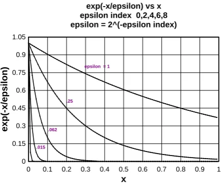
characterized by a small parameter appearing in the differential equation. For example consider the function exp (-x/ ε) which qualitatively exhibits localization characteristics of solutions typical of these types of boundary value problems. It is plotted in fig. 1 for various values of ε
from which the behavior of the function in a region near x=0 can be seen. It is clear that to accurately represent this function by a set of points, a sufficient number of points needs to be in the localized region itself.
x
exp(-x/epsilon)
exp(-x/epsilon) vs x epsilon index 0,2,4,6,8 epsilon = 2^(-epsilon index)
0 0.1 0.2 0.3 0.4 0.5 0.6 0.7 0.8 0.9 1
0 0.15 0.3 0.45 0.6 0.75 0.9 1.05
epsilon = 1
.25
.062
[image:1.595.319.536.344.524.2].015
Fig. 1. The function exp (-x/ ε) is plotted as a function of x over the interval (0, 1) illustrating its localization near x=0 for small epsilon.
One method of solution, known as the uniform mesh method, is to simply place a uniform mesh over the interval which would require for sufficiently small epsilon an inordinate number of points resulting in excessive relaxation times. The limitations of the uniform mesh method are well known [3].
Another method is to allowing the mesh spacing to vary throughout the net thus providing a high density of mesh points in the localized region. This method was in fact the first technique to be applied to this problem and goes under the name of “fitted meshes”, “non uniform meshes”, or “Bakhvalov fitted meshes”, is described in [3] and is a method currently used by many workers in the field [8]. It is a method capable with appropriate parameter adjustments of reasonably high accuracy (~10-9) although issues
surrounding this technique have been discussed in Farrell et al [3] and revolve around its complexity particularly when application is made to higher dimensional problems. Thus the higher precision of this method comes at a cost of increased
High Precision Calculations of One Dimension
Singularly Perturbed Boundary Value Problems
Using Multi Region FDM
complexity.
A significant advancement to the field came in ~1988 by Shishkin [5] who split the region into two non overlapping, separately uniform sub regions, the first being containing the rapidly varying portion of the function onto which ~N points were placed thus giving this region a very high density, and the second containing the very slowly varying portion of the function onto which again N points were placed. This two region structure led to solutions in both regions (resultant precision of ~10-5) and allowed to some extent the boundary
layer itself to be determined. The only problem remaining was the matching between the two regions. The matching problem is of course non trivial and has been the subject of a large amount of research over the ensuing 20 years being yet today a field of active research [4, 5, 10]. To date precisions in the range 10 -4 to 10-6 have been achieved.
Somewhat prior to the time that Shishkin developed the two region solution to the one dimensional singular problem, a multiregion technique was developed by the author [12] to solve a similar type of problem in two dimensions related to the calculation of electrostatic potentials in cylindrically symmetric geometries constructed using rectangular elements (as rings of rotation). In this situation the differential equation is the 3 dimensional Laplace’s equation which is reduced to a two dimensional problem as a result of the problem symmetry. While the differential equation itself contains no small parameter and hence is itself non singular, the function which is its solution for geometries created using the rectangular elements has singularities near the corner points of those elements. These geometrically induced singularities create large algorithmic errors in their vicinity which propagate throughout the net. These errors were found to be mitigated by creating a set of regions telescopically converging to the respective singular points and thus provided the first instance of multi region FDM (finite difference method) to a problem with “singular point” difficulties [12]. This work has been continued, refined and is reported in a recent series of publications [13-16].
It is believed that workers in the areas of singularly perturbed boundary value problems and electrostatic potential calculations were completely unaware of each others existence even though their research efforts coexisted in time. This changed in 2008 at a multi disciplinary conference which the author attended when a paper was presented by R.K.Bawa [5] making the author aware of the singularly perturbed one dimensional boundary value problem (SPBVP). The strong possibility that the method used in the electrostatic situation would be applicable to this problem was quickly recognized since both of these problems were had localized singularities.
This paper is a result of that recognition.
To provide an overview of this paper and to help keep track of its logical flow the following outline is provided. 2. Technical concepts
2.1 The single region FDM process 2.2 Algorithm development 3. The multi region structure 3.1 Region definition
3.2 Manually creating a region structure 3.3 Relaxing a region structure
4. Auto establishing a multi region structure. 5. Basic tests to corroborate the technique
5.1 Convergence of the multi region nets with respect to c13_c
5.2 Stability
6. Multi region FDM solutions for ε between 1 and 2-60
7. The dependence of single point algorithmic errors on c13_c
8. Generalized applicability 9. Notes of caution.
10. Comparison with other methods. 11. Conclusion
The test example is:
(1) εd2u/dx2 + du/dx = 0, u(0)=0, u(1)=1
It is one of the simplest examples of a singularly perturbed boundary value problem and an example from class 2.1 of Farrell et al. [3] having also been recently studied by Bawa [5]. This example is one which has been typically used by workers when presenting a new technique. Its simplicity allows the easy abstraction of the technique’s main features while providing a basis for application to more complex problems. That it has a known solution allows for the immediate verification of numerical results.
2. TECHNICAL CONCEPTS
The technical concepts required for understanding the multi region FDM process are twofold; 1 a knowledge of the basic single region relaxation process; 2 an understanding of the algorithm development method.
2.1 THE SINGLE REGION FDM PROCESS
The single region FDM process is explained in many texts [17, 18] and presented here to standardize our terminology in preparation for its extension to multi regions.
The domain of u(x) will be transformed to one having n equally spaced subintervals within the boundary points occurring at 0 and n. This single region may then be relaxed by stepping through the n-1 points of the interval, at each point updating its value using values of its surrounding points by means of an algorithm. For the one dimension problem values of two points are required by the algorithm, the values taken from the immediately preceding and succeeding mesh points. This process is repeated throughout the interval, the repetition iterated until an appropriate stopping criterion is reached at which time it is said that the solution has converged. This type of convergence will be called iteration
convergence to distinguish it from other types of
convergence.
2.2 ALGORITHM DEVELOPMENT
During the relaxation cycle an algorithm is required at each mesh point which, using values at its surrounding points will yield an accurate value of u at the point itself. In order to create an interval with n subintervals, the interval [0,1] is transformed by the substitution of x = z/n.
Applying this transformation to (1), the following is obtained:
(2) nε d2u/dz2+ du/dz = 0, u(0) = 0, u(n) = 1
mesh point, a final substitution is made, z = r + ri with r being
the relative coordinate of the point z with respect to the mesh point at z = ri. Thus one obtains:
(3) nεd2u/dr2+ du/dr = 0, u(0) = 0, u(n) = 1
A power series representation of u about a mesh point at rj
on the z axis is written:
(4) u(r) = c0+c1r+c2r2+… +cjrj +O(rj+1 )
Where O(rj+1) indicates that terms in (4) containing powers
of r larger than j are neglected.
Defining the order of the algorithm as the highest included power of r in the power series representation of u from which the algorithm is derived, the above power series describes a power series of order j used in the development of a jth order algorithm.
The actual process of algorithm development from its power series representation may again be found in elementary texts on differential equations [17, 18] and hence only an abbreviated description will be given for an order 5 algorithm. This may be useful to those unfamiliar with this classical technique and will render understandable the remainder of the paper. From this example it is seen that the process can be easily generalized to the development of higher order algorithms.
Using (4) the 5th order power series representation of u is
written:
(5) u(r) = c0+c1r+c2r2+c3r3+c4r4+c5r5 + O(r6)
To find u(r) the 6 coefficients, c0.. c5 need be determined.
This is accomplished in the following manner: First the differential equation (3) is evaluated using the representation of u given in (5) which results in a single equation again being a power series in r:
(6) (c1+2nεc2)r0 + (2c2+6nεc3)r1 + (3c3+12nεc4)r2
+ (4c4+20nεc5)r3 + O(r4) = 0
Since (6) is true in an arbitraryneighborhood of r=0, each coefficient of rj is required to be 0, and results in 4 equations.
As there are 6 unknowns two additional equations are required. They are found from evaluating u(r) at 2 surrounding meshpoints, in this instance taken from mesh points on either side of r=0. Letting b5 = u(r=1) and b1 = u(r=-1) we have the following set of 6 linear equations which may be solved for c0 .. c5.
b5 = c0+c1+c2+c3+c4+c5
b1 = c0-c1+c2-c3+c4-c5
(7) c1+2(nε) c2 = 0
2c2+6(nε) c3= 0
3c3+12(nε) c4= 0
4c4+20(nε) c5= 0
The complete solution of this linear equation set is listed below both to illustrate the order of the complexity of the 5th
order algorithm and to emphasize the fact that the algorithm development process may actually determine the complete set of coefficients (c0... c5). This ability will permit the
definition of the c13 in §4. It will also enable by the use of (5),
an interpolation for values between mesh points. The solution is:
c0 = (+120(nε)4*b1+120(nε)4*b5-
60(nε)3b1+60(nε)3b5+20 (nε)2b5+20(nε)2b1+5(nε)b5-
5(nε)b1 + b1 + b5)/ (+240(nε)4 + 40(nε)2 +2 )
c1 = (-60(nε) 4*b1+60(nε) 4*b5)/(+120(nε) 4+20(nε)2+1)
(8) c2 = (+30(nε)3*b1-30(nε)3*b5)/ (120(nε)4 + 20(nε)2
+ 1 )
c3 = (+10(nε)2*b5-10(nε)2*b1)/ (+120(nε)4+20(nε)2+1)
c4 = (+5(nε)*b1-5(nε)*b5)/ (+240(nε)4+40(nε)2+2)
c5 = (+b5-b1)/ (+240(nε)4+40(nε)2+2)
In general to determine a jth order algorithm, one applies the differential equation (1) to a jth order power series which results in a power series of order j-2 due to the d2u/dr2 term in
the differential equation. As there are j cj’s to be determined
an additional two equations are required as in the example above. This is in contradistinction to the situation in 2 dimensions where the 5th order algorithm developed for the
cylindrically symmetric electrostatic, has 21 coefficients, while the number of equations resulting from the application of the differential equation to the power series is only 11. Thus an additional 10 equations are required and are obtained from the 10 surrounding meshpoints. It is further noted that the number of required meshpoints for the two dimensional case grows rapidly as the algorithm order increases, requiring for example 21 surrounding meshpoints for the order 10 algorithm. (Algorithm development is considerably simpler in one dimension.)
The consistency of the set of equations (8) from which the solutions are obtained must be established for each individual differential equation. For all of the algorithms that have been determined for this and other one dimensional examples, no inconsistent situations were found. This was not the case however in two dimensions where a sufficiently unsymmetrical set of mesh points would result in an inconsistent equation set.
It is noted that the notation using b1 and b5 for the mesh points to the left and right of the central meshpoint has been chosen to be consistent with the notation previously employed [13-16].
3. THE MULTI REGION STRUCTURE
3.1 REGION DEFINITION
A region is considered to consist of an interval containing its mesh points and to have both a single parent region and possibly many child regions. It is required to be contained within its parent and have an enhanced density with respect to its parent. The region may be represented by the following notation:
index, parent index, left endpoint, width, subintervals; where width is the width of the interval in parent units, and subintervals is the number of subintervals in a single parent interval. Thus a region has the following characteristics: 1. every region except the main net has a parent and is contained within the parent; 2. a region may have child regions, and for those child regions it is their parent; 3. child regions are non-overlapping. It is noted that each region has a number of points N in its interval and an effective n, neff, which is found from multiplying the neff of
the parent times its subintervals value. (neff of the main net is
its number of mesh points.)
3.2 MANUALLY CREATING A REGION STRUCTURE
to be much higher there than in other places in the net. Thus a 3 region structure which puts an enhanced density in the vicinity of x = 0 having the above parameters can be manually created and is listed below:
0,-1, 0, 32, 1 (9) 1, 0, 0, 3, 4 2, 1, 0, 3, 4
(This structure has been found to have a precision of 3*10-8 for ε= 2-10.)
3.3 RELAXING A REGION STRUCTURE
Any region within the structure is to be relaxed with the standard single region FDM process described in 2.1. The multi region relaxation process will proceed in the following manner: 0 regions within the structure are sequential relaxed; 1 before a region is relaxed its boundary points are copied from their image points in the parent region; 2 no point in the region is relaxed which is either on a boundary or has an image in a child region; 3 after a region is relaxed, the image points within it of its parent are copied into its parent. The process is terminated when a given stopping criterion is reached.
In this manner a region structure can be created for any ε, relaxed, and its precision determined. The process can be continued by trial and error until the desired precision is obtained. The problem with the above is the requirement for significant user intervention during the process. To overcome this, a procedure for auto establishing a region structure has been developed and is described in §4 below. It will be shown that for a desired precision the required multi region structure can be auto established thus removing user intervention from the process.
4. AUTO ESTABLISHING A REGION STRUCTURE.
Let us suppose that we have a base region which has been relaxed, and that it is desired to add a child region to this base region which will improve the overall precision of the solution. The task is thus to construct a child region to contain the mesh points of the base region having high algorithmic errors. The algorithmic errors for these mesh points in the child region will then be reduced from their errors in the parent due to the enhanced density of mesh points in the child. The task thus becomes to determine those points in the base region which would have high algorithmic errors from the values of the mesh points themselves. The above would be accomplished if one could estimate the algorithmic error at a mesh point from the values of its
neighbors. This estimation will be made possible by the use
of |c13(z)|, c13 (z) determined during the development of the
order 13 algorithm. (Note that the functional dependence of c13 on z arises from the dependence of c13 on b1 and b5 which
themselves are functions of z.
The motivation for using |c13| as an algorithmic error
estimator is given in the following qualitative argument: The truncation error in evaluating c0 using an order 13 algorithm
will involve coefficients c14 and above, all of which are likely
to be of the order of magnitude of c13 or smaller. Thus it is
not unreasonable to expect that the single point algorithmic error at a mesh point would be of the order of this quantity. It must be emphasized that at this point the above is simply an assumption whose validity needs to be examined (see §7).
Let c13_c be the desired precision of the numerical
solution. The region may be then divided into two sets, one having their |c13| values less than the desired precision and the
other greater than the desired precision.
Using the above concepts the region structure is created as follows: first N is selected for the main net and the main net relaxed. After this relaxation |c13| values are determined
for all points in the main net and those having a |c13| of < the
desired precision are colored blue, the remainder green. (N is initially chosen for the main region so that some blue points are in the region.) A child region is then constructed so that it contains all of the green points. The interval between parent points in the child region is divided into say s subintervals (fixed at 4). The region structure now consists of a parent net and one child region (for only one contiguous set of green points) or many child regions (for several separately contiguous sets of green points).
Without loss of generality suppose only one child region was found. The relaxation of the current two region structure (parent and child) proceeds previously described. After it has been relaxed a child region may be added to the two region structure again using desired precision to divide the mesh points of the region into two sets. The added region would be a child region of the previous child region which would be its parent. The 3 region structure is then relaxed, the region construction being continued until the last child region has no points with |c13| values > the desired precision. At this point
the structure is complete and a final relax of the region structure is made using possibly a more stringent end criterion than used during the region construction. It should be noted that both the location of the singularity as well as the number of singularities are determined by the process itself and the process is self terminating.
It will be later be shown in §7 that for our example, c13_c
(the desired precision) is in fact an upper bound to the single point algorithm error for all mesh points having |c13| values
less than it. Thus the above region creation process has the following characteristic: during the final relax cycleno point in the mesh is relaxed that has a single point algorithmic error greater than c13_c and hence apart from the cumulative round off errors which occur, the precision at any point with the entire structure should be of the order of or
less than c13_c. Thus a structure can be created which at the
end of the final relaxation will give a maximum error at any mesh point within the net of the order of or less than the desired precision. And the only user input is the desired precision of the final result. It is noted that this type of process is also termed adaptive.
5. BASIC TESTS TO CORROBORATE THE TECHNIQUE
considerable confidence) and the solution using the new multi region FDM technique.
In much of the literature, particularly those methods based on the piecewise uniform method of Shishkin, the order of convergence of the process is a quantity often determined for the process. It may be calculated from:
(10) emax = a*np ,
where emax is the maximum error of the numerical solution parameterized by n, the number of mesh points. The
order of the convergence is then defined as –p. For Shishkin
related methods the number of meshpoints is taken to be the number of points in the main net.
Unfortunately any definition of the order of convergence of a process dependent on number of mesh points does not apply to the multi region FDM process described here since in most instances the region structure created with differing values of c13_c (desired precision) for a given ε will have the
same number of regions and hence a identical neff for all the
regions (including the main net) but its after relax precision will differ markedly depending on c13_c. However, in order
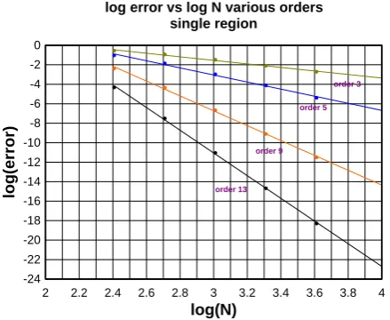
to examine the order of convergence of the high order algorithms in a defining context, the algorithms will be used in a single region FDM relaxation problem from which the order of convergence is well defined and can be evaluated using (10). To this end ε is chosen to be 2-10, nets created
[image:5.595.318.537.422.600.2]having varying number of mesh points N (from 256 to 8192), relaxed using a particular algorithm, and emax and hence p determined for each algorithm. The results are plotted in Fig. 2 for algorithms of order 3, 5, 9, 13.
log(N)
log(error)
log error vs log N various orders single region
2 2.2 2.4 2.6 2.8 3 3.2 3.4 3.6 3.8 4
-24 -22 -20 -18 -16 -14 -12 -10 -8 -6 -4 -2 0
order 13 order 9
order 5 order 3
Fig. 2. The log of the single region error for ε = 2-10 is shown as a function
of the log of the number of mesh points in the net for various order algorithms used in the relaxation process. The slopes ranging from ~ -11 for the order 13 algorithm to ~ -2 for the order 3 algorithm give the order of convergence of the algorithm.
From the slope of the error curves (the 8192 net is used as the reference) the order of convergence of the particular algorithm can be determined. The table below gives the order of convergence for the various algorithms.
algorithm Order of convergence order 3 1.82
order 5 3.6437 order 9 7.63689 order 13 11.65862
Seen from the above table is that the high order algorithms have large orders of convergence, and hence are suitable for the relaxation process. It is seen also that orders of convergence increase in an essentially linear manner with respect to the order of the algorithm.
From the order 13 curve in Fig. 2 it is seen that; 1 the nets converge as a function of N to the 8192 net and 2; the precision of the 8192 net (log (N) ~ 3.9) can be estimated to be ~10-22 for ε = 2-10.
5.1 CONVERGENCE OF THE MULTI REGION NETS WITH RESPECT TO C13_C (THE DESIRED PRECISION VALUE)
From the discussion above, it was seen that n is not and cannot be made to be a useful parameter in determining convergence properties of the multi region process. Thus another parameter needs to be determined. Defining cut by:
(11) cut = log10 (c13_c)
It will be shown that cut is in fact a convergence parameter. One can see that cut is a parameter of convergence by considering a problem (ε = 2-10) for which we have a
reference net (the single region 8192 net) and then creating and relaxing a number of multi region structures for various cuts.
Fig. 3 shows the resultant plot from which it is seen that the multi region solution converges and converges to the 8192 solution as cut is decreased from -6 to -20 thus demonstrating that cut is a convergence parameter. This also demonstrates the overlap of the multi region solution with that of a single region solution for a common problem, ε = 2-10, since as seen
in Fig. 3 the multi region solution converges to the 8192 solution.
cut
log max difference
log error vs cut
converging to single region 8192 net epsilon = 2^(-10)
-22 -20 -18 -16 -14 -12 -10 -8 -6
-22 -20 -18 -16 -14 -12 -10 -8 -6
Fig. 3. Seen in this figure is that the multi region process for a given cut converges to the 8192 single region reference net thus showing that cut is a convergence parameter.
5.2 STABILITY
[image:5.595.60.280.423.603.2]converges to is not stable(see definition below). 5.2.1 DEFINITION OF PROCESS STABILITY.
A net is considered having been relaxed from an arbitrary initial state with appropriate boundary conditions using a process. The process consists of an iteration method coupled with an algorithm used in the process to determine the values of the function at each mesh point from the surrounding points. The process is considered to be stable if the following two conditions hold: i. The process converges to a final state, uN(z). ii. The iteration process starting from any perturbation
of the final state must converge to the same final state, uN(z).
5.2.2 THE SIMULATION METHOD USING MONTE CARLO TECHNIQUES
Defining Z (z) as the solution to (1) with Z (z) =0 for all z, it is a straightforward exercise to show that uN(z) is stable if Z
is stable. We will determine the stability of Z and hence uN
by constructing random initial states for Z (all non boundary mesh points values are chosen randomly from the interval [-1, 1]) and then relaxing Z for each of these states. If the relaxation converges to Z for every random initial states in a sufficiently large simulation set it is considered to be stable. From equation (5) it is seen that the value c0 depends
linearly on b1 and b5 (this is true for all algorithms as well as the 5th order algorithm). Calling the coefficients of these
quantities cb1 and cb5, c0 may be written: (11) c0 = cb1*b1+cb5*b5
It is noted that the coefficients cb1 and cb5 depend upon the particular algorithm used in the relaxation process and that in any multi region structure only a small number of cbj values are actually realized (cb1 and cb5 are constant throughout each region depending only on nε, where n is the effective n for the region).
The process simulation will be treated in two steps. First values of cb1 and cb5 will be scanned from -2 to 2 and the stability of each pair (cb5, cb1) determined. This will provide a plot of the stable values of cb1 and cb5. The realized values cb5, cb1, obtained for a particular algorithm will be superimposed upon the stability plot thus determining the stable points of the algorithm.
5.2.3 RESULTS FROM THE SIMULATIONS
The perturbed Z net was created by constructing a single region mesh having N mesh points. The values at all non boundary points are initialized to random numbers in the range -1 and 1 with the boundary points being set to 0. (It should be noted that for any region in the multi region structure the N to be used for its stability determination is the number of points in its interval and not its effective n defined in §3.1.) This net was then relaxed and found stable if the value at every mesh point was less than 10-15 for iterations
larger than a given number. It is noted that for this situation a mesh point was either stable or reached a sufficiently large value during a relax cycle at which point the process was terminated. Only in other cases (mesh points used in the algorithm not b1, b5) did the simulator find the very special situations in which either the entire net would relax to a non zero function or successive iteration cycles would give alternate signs to the non zero function and so in fact would never satisfy the end criterion, i.e. it would never become unbounded but never converge. The stability plot for a j trial simulation set is the intersection of all of the individual
[image:6.595.316.532.166.343.2]simulation plots. A single simulation consisted in finding the stability of each pair (cb5, cb1) in its domain using the same random initial function for the mesh point values.
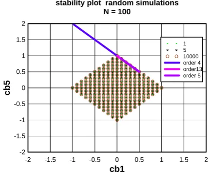
Fig. 4 shows a plot of the final stability region for a 100 point mesh for the simulation sets containing 1, 5, and 10000 trials. Seen that the final stability region does not change after the first ~1-5 simulations and hence implying that only a small number of actual simulations are in fact required to determine the final state of the stability plot.
cb1
cb5
stability plot random simulations N = 100
-2 -1.5 -1 -0.5 0 0.5 1 1.5 2
-2 -1.5 -1 -0.5 0 0.5 1 1.5 2
1 5 10000 order 4 order13 order 5
Fig 4. Seen is that the stability plots for a 100 point net for 1, 10 and 10000 simulations are equivalent. Also plotted are the possible values of cb1 and cb5 for the various algorithms for nε between .0001 and 10 showing that the odd order algorithms are stable for all nε while the order 4 algorithm has is unstable for a range of nε values.
The quantities cb1 and cb5 in a relaxation process are determined by the particular algorithm used. The algorithms developed from (1) depend only on nε (n is the neff for the
region). By scanning nε over its domain (.0001 to 10), the set of realized pairs (cb5, cb1) can be determined for each algorithm. Thus superimposed on the plot in Fig. 4 are the pairs (cb5, cb1) for algorithms of order 5 and 13 (order 9 was similar). Seen is that all possible pairs (cb5, cb1) produced by these algorithms lie within the stable region of the stability plot and hence the solutions using orders 5, 9, and 13 are stable for all values of nε. Shown also is a plot of the pair (cb5, cb1) for an order 4 algorithm which is seen to be unstable for a range of nε values (nε <~.3) but stable otherwise. This type of behavior has occurred for other even order algorithms and it is believed that even order algorithms have regions of instability while odd order algorithms are stable.
It may be useful to point out that: 1 having an algorithm with an unstable region does not preclude its use in its stable regions, and 2 the algorithm stability will need be determined for each problem individually. In other examples selecting the mesh points to be the two points immediately to the right or left of a central point has produced algorithms with unstable regions and points in the unstable regions which both oscillated and were bounded and convergent.These algorithms, however, are quite useful to the relaxation process when used in their stable regions and in order to use them it is essential to be able to determine their regions of stability.
together with its detailed relaxation schema. This has been done and the results have found that the multi region process is stable when it uses stable algorithms.
§6. MULTI REGION FDM SOLUTIONS FOR EPSILON BETWEEN 1 AND 2-60
Let epsilon index be defined by: (12) epsilon index = -log2 (ε)
To establish the appropriate structure for a desired epsilon, one starts with epsilon index of 0 and establishes its multi region structure as described in §3. Using this structure as the basis for the next epsilon, epsilon index is incremented by 1 and the multi region structure for this new epsilon is determined. This is continued until the structure for the final epsilon has been created. As an example the region structure for ε = 2-40 (~10-12) having a required precision of 10-16 has
been found to be: 0, -1, 0, 32, 1 1, 0, 0, 15, 4 2, 1, 0, 15, 4 …… 19, 18, 0, 15, 4
where the fields are defined in §3.1. (Values other than 4 for the number of child subintervals in a parent interval have been tried and found to have essentially little effect on either the final precision or relaxation time.)
It is found after determining and relaxing the above structure (using double precision arithmetic, lsb of ~10-16),
that the maximum error at any point within the structure was 2.9*10-14 which occurred in the above example in region 19,
z = 17. Since it was suspected that the above error was dominated by the cumulative effect of round off errors of the double precision arithmetic, the final net was relaxed using a very high precision software arithmetic unit. After the net was relaxed using the high precision code the maximum error was found to be 4.01*10-18 both confirming the suspicion that
the excessive error was due to round off and likely giving a very good estimate to errors due to the relaxation process itself. (In the following the high precision code will always be used during the final relax of the multi region structure.) The above structure would by construction be valid for any epsilon <= 2-40.
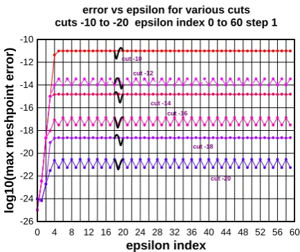
Thus for any epsilon a region structure can be determined, relaxed and the maximum net errors found and plotted vs epsilon. Such a plot is shown in Fig. 5 for various cuts. (The errors have been determined using the known exact solution as the reference.) Epsilon index is incremented by 1 for most points within the epsilon index range 0-60 except for points between 18 and 20 where the increment was taken as 0.1 and is plotted as the darkened curve in the Fig. 5. Seen is that the maximum mesh point error shows slight periodic variations (periodicity 2) within the range 10 to 60. It is noted that if epsilon index increment was 2 all curves would appear to be exactly constant which would be an artifact of the periodicity of 2. Seen also in fig. 5 is that precisions in excess of 10-20
can be obtained with appropriately large negative cuts.
epsilon index
log10(max meshpoint error)
error vs epsilon for various cuts cuts -10 to -20 epsilon index 0 to 60 step 1
0 4 8 12 16 20 24 28 32 36 40 44 48 52 56 60
-26 -24 -22 -20 -18 -16 -14 -12 -10
cut -10
cut -12
cut -14
cut -16
cut -18
cut -20
Fig. 5. The maximum error at any point in the net is plotted vs epsilon index for various cuts. Shown also is a higher precision plot between epsilon index 18-20. Seen is that the error is periodic in epsilon index with period 2 units, while the phase is not independent of the cut, thus the apparent constancy of the cuts -10, -14, -18.
As mentioned above algorithms of order 13 were used in all of the mesh relaxation calculations. To see the dependence of the resultant error on algorithm order, epsilon was set at 2-20; the required structure created using the order
13 algorithm and relaxed using algorithm orders of 5, 9, and 13. The resultant plots are shown in Fig. 6.
cut
log10(maximum error)
maximum error vs cut for various orders for epsilon index = 20
-22 -21 -20 -19 -18 -17 -16 -15 -14 -13 -12 -11 -10 -9 -8
-22 -20 -18 -16 -14 -12 -10 -8 -6 -4
order 5
order 9
[image:7.595.319.536.51.233.2]order 13
Fig. 6. The maximum error in the mesh for ε = 2-20 are plotted vs cut for
orders 5, 9, and 13. Seen is the marked dependence of error on order for high precision cuts whereas for low precision cuts the errors tend to converge.
Seen is the marked sensitivity of precision on the algorithm used. This plot also shows that for cuts ranging from -8 to -20 the precision of the 5th order algorithm varies
between 10-4 and 10-7 while the order 13 algorithm varies
between 10-12 and 10-20 thus emphasizing that the advantages
of multi region FDM are only fully realized with the accompanying use of high order algorithms.
7. THE DEPENDENCE OF SINGLE POINT ALGORITHMIC
ERRORS ON C13_C.
At this point we have a reference net (cut = -20) for the multi region solution for epsilon in the range of 1 to 2-60.
point algorithmic error can be plotted vs |c13| for all points in
the net. Note that in such a plot, all of the mesh points in the net are represented on the |c13| axis. Such a plot is shown in
Fig. 7 in which N and epsilon are scanned from 32 to 256 and 20 to 2-12 respectively. The plot is made for an order 13
algorithm. It was assumed in §4 that the single point error at a mesh point would be of the order of |c13| which from Fig. 7 is
seen to be valid. In addition it is seen that statement can in fact be strengthened to: at any meshpoint z the algorithmic
error is bounded above by |c13(z)|. The function represented
by this upper bound is called the maximum error function which is a function of the mesh point location z and is also shown in Fig. 7.
To summarize, any point within the net has a calculatable value of c13 and hence a value of the maximum error function
[image:8.595.318.542.53.233.2] [image:8.595.60.293.274.454.2]of the point can be determined. Thus Fig. 7 shows that its single point algorithmic error value will be less than its maximum error function value.
log|c13|
log (algorithm value - theory value)
single point algorithm error vs c13 N from 32 to 256, epsilon index 0 to -12
-26 -24 -22 -20 -18 -16 -14 -12 -10 -8 -6 -4
-26 -24 -22 -20 -18 -16 -14 -12 -10 -8 -6 -4
data points max error function
Fig. 7. The errors in evaluating an algorithm order 13 are plotted vs log (c13). All points within the net are on the log|c13| axis. Seen is that the maximum error function is an upper bound to the single point algorithmic error for any mesh point in the net.
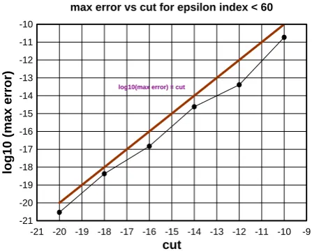
In fig. 8 the maximum errors in relaxed net for any epsilon in the range 10 to 60 are given for various cuts. Seen is that the max errors are in fact less than cut as anticipated by the discussion above. The implication of this is that one can create a region structure based on a desired resultant precision and the relaxed structure will in fact meet or exceed the desired precision. It is clear in fact that the region structure created is in fact optimal in that this structure is the smallest structure having the desired precision.
cut
log10 (max error)
max error vs cut for epsilon index < 60
-21 -20 -19 -18 -17 -16 -15 -14 -13 -12 -11 -10 -9
-21 -20 -19 -18 -17 -16 -15 -14 -13 -12 -11 -10
log10(max error) = cut
Fig. 8. The log10 (maximum error) for 60>epsilon index >10 are plotted vs cut. Seen is that the measured values are less than cut
For a particular cut one can anticipate that the maximum errors only be of the order of the of the maximum error function since there could be a cumulative effect of those errors (which are strictly not round off errors) so that the maximum error value for a given epsilon could be slightly larger than the maximum error function. Thus that the errors found are less than the maximum error function is fortuitous but not required.
8. GENERALIZED APPLICABILITY
The establishing of the region structure is clearly not dependent on a priori knowing the location of the singular point since during region creation one simply finds all those points with |c13| values greater than a given value and then
defines a child region containing those points. The singular point itself could be anywhere within the interval (0, 1). By the same token if there were more than 1 singular point the process would both find and isolate those points.
As the method is a derivative of the two dimensional electrostatic problem, the extension of the technique to two dimensions has already been demonstrated [12-16]. It should be apparent that the technique does not depend upon knowing the origin of the singularities i.e. the differential equation or the geometry but only on the behavior of the function produced by the combination of both. Child regions are simply placed in over those points at which the single point algorithm precision would exceed a certain value regardless of the “cause” of the singularity (a small parameter in the differential equation or near an edge of a rectangular element) in this way assuring that during the final relaxation process the algorithm is only applied to those points whose single point precision is less than or equal to the desired precision.
9. NOTES OF CAUTION.
0. The result is not epsilon uniformly convergent, since the structure established for the epsilon index = 60, for example, would require for the same precision a different structure if epsilon index were larger than 60. It is not felt that this is a real limitation of the technique since the structure for epsilon index = 60 would cover all epsilons in the range 2-60 (`10-18)
to 1 which would likely encompass any realizable physical modeling situation.
technique will be viable. Algorithm development is however only assured for linear differential equations. Algorithm development for non linear equations may be possible but there is no assurance of success.
2. During the algorithm development process a set of linear equation must be solved. If the differential equation producing this equation set contains a large number of constants, the linear solver may have difficulties solving the resultant equation set. Its success would then depend on the sophistication of the solver.
3. The high precision result described herein comes at a price and the price is time. For example, to create and relax the multi region structure using the built in double precision arithmetic unit of the processor, for epsilon = 2-60 with a cut
of -20 takes ~350 seconds while relaxing this output with the high precision software takes an additional 300 seconds. This is not considered to be excessive but it is certainly not instantaneous. It is also noted that the linear equation set for the high order algorithms were solved in the same time interval.
10. COMPARISON WITH OTHER METHODS.
There are three methods with which this technique can be compared: the piecewise uniform mesh method of Shishkin method, the fitted mesh method of Bakhvalov, and the multi grid method.
10.1 PIECEWISE UNIFORM MESH METHOD.
This method has only two regions, a high density region in the localized region of the function and a low density region in the rest of the net. Within each region there are a sufficient number of mesh points to mitigate the algorithmic errors for points within the region. The problem is of course the link between the two regions. It is felt that to accurately link the two regions either a variable mesh might be used or the multi region structure developed here used. If neither of these is used then it is unlikely that this method will produce precisions much higher than workers have already obtained. However, if accuracy is not an issue, it is not only applicable but probably preferred.
10.2 FITTED MESH METHOD.
The fitted mesh method uses a variable mesh which is capable of putting a very high density in the localized region of the function. There is a clear equivalence of this method and the multiregion method discussed here in that if the mesh density at any point net of the fitted mesh was of the same order as the density at the equivalent point in the multi region net the single point errors would in fact be similar if the single
point algorithm precisions were themselves equivalent. (See
Fig. 6). Thus the fitted mesh method could have precisions equivalent to those of the present technique.
10.3 MULTI GRID FDM.
Multi grid is in extensive use in a wide variety of applications. However a literature search of multi grid applied to the test example above has located only two references [7, 19] with precision data in the 10-7 range.
However due to the wide ranging concept of multi grid it is certainly capable of having the same structures as those determined here. And if it does have the same structures and its single point algorithms have equivalent precisions as the
order 13 algorithm developed here then the precisions of the
two methods should be the same.
Thus both the fitted mesh method and the multi grid method are capable of high accuracy and could be competitive with the multi region method developed here. It is believed however that the simplicity of the multi region method would compete rather strongly against complexity of either for problems of common applicability.
11. CONCLUSION
The multi region FDM method has been described and applied to a one dimensional problem of singularly perturbed differential equations. The following have been demonstrated: 1 for epsilon in the range of 1 to 2-60 precisions
of the order of ~10-20 can be achieved. 2 the required region
structure can be auto established.
The advantages of the technique are two fold. The first is its simplicity. It uses the standard single region relaxation techniques along with well known classical algorithm development processes. The second is its performance. It has been shown capable of achieving precisions which are many orders of magnitude beyond those which have been obtained by other techniques. The combination of these two properties should make it a useful addition to the techniques available for solving singularly perturbed boundary value problems.
Newark, VT Oct 13 2008
ACKNOWLEDGMENT
It is with very great pleasure that I acknowledge the help R.K.Bawa who during his presentation at the IMECS2008 introduced the author to the (hitherto unknown) field of singularly perturbed boundary value problems and was supportive during all stages of this research.
REFERENCES
[1] N. S. Bakhvalov On the optimization of methods for boundary value
problems with boundary layers. J. Numer. Meth. Math. Phys. 9 (1969)
841-859 (in Russian).
[2] H.-G. Roos, M. Stynes, L. Tobiska, Numerical Methods for Singularly
Perturbed Differential Equations. Springer, Berlin, 1996.
[3] P. A. Farrell, A. F. Hegarty, J. J. H. Miller, E. O’Riordan, and G. I. Shishkin, Robust Computational Techniques for Boundary Layers, Chapman & Hall/CRC Press, Boca Raton, 2000.
[4] S. Natesan, R. K. Bawa, C. Clavero, Uniformly Convergent Compact Numerical Scheme for the Normalized Flux of Singularly Perturbed
Reaction-Diffusion Problems, International Journal of Information and
Systems Sciences, 3 (2007) 207-221.
[5] R.K.Bawa, V. Kumar, An ε-Uniform Initial Value Technique For
Convection-Diffusion Singularly Perturbed Problems, Proceedings of
International MultiConference of Engineers and Computer Scientists 2008, Hong Kong, 19-21 March, 2008.
[6] M.K. Kadalbajoo, K.C. Patidar, A survey of numerical techniques for
solving singularly perturbed ordinary differential equations, Appl. Math.
Comput. 130 (2002) 457–510.
[7] D. Kamowitz, Multi grid applied to singular perturbation problems, Appl. Math. Comput. 25 (1988) 145–174.
[8] Relja Vulanovic, Special Meshes and Higher-Order schemes for
singularly perturbed boundary value problems, Novi Sad J. Math. 31 (2001)
1-7.
[9] G. I. Shishkin, Grid Approximation of Singularly Perturbed Parabolic
Equations with Internal Layers, Sov. J. Numer. Anal. Math. Modeling, 3
(1988) 392-407.
[10] C. Clavero, J. L. Gracia, F. Lisbona, High Order Methods on Shishkin Meshes For Singular Perturbation Problems of
Convection-Diffusion Type, Numerical Algorithms 22 (1999) 73-97.
[11] R. Vulanovi, The layer-resolving transformation and mesh
Computational and Applied Mathematics 203 (2007) 177 – 189.
[12] D. Edwards, Jr., Accurate Calculations of Electrostatic Potentials for
Cylindrically Symmetric Lenses, Review of Scientific Instruments, 54 (1983)
1229-1235.
[13] D. Edwards, Jr., High Precision Electrostatic Potential Calculations
For Cylindrically Symmetric Lenses, Review of Scientific Instruments, 78
(2007) 1-10.
[14] D. Edwards, Jr., High precision multiregion FDM calculation of
electrostatic potential, Advances in Industrial Engineering and Operations
Research, Springer, 2008, ISBN: 978-0-387-74903-7.
[15] D. Edwards, Jr., Accurate potential calculations for the two tube
electrostatic lens using a multiregion FDM method, Proceedings
EUROCON 2007, Warsaw, Sept.9-13, 2007.
[16] D. Edwards,Jr., Single Point FDM Algorithm Development for
Points One Unit from a Metal Surface, Proceedings of International
MultiConference of Engineers and Computer Scientists 2008, Hong Kong, 19-21 March, 2008.
[17] Erwin Kreyszig, Advanced Engineering Mathematics, John Wiley and Sons, New York, 1962.
[18] Murray Spiegel, Applied Differential Equations, Prentice-Hall, New Jersey, 1958.