Abstract—In bridge design practice, especially in case of large span bridges, wind loading can be extremely dangerous. Since the collapse of the Tacoma-Narrows Bridge in 1941, bridge flutter assessment has become a major concern in bridge design. In the early ages, wind tunnel tests were made in order to assess the aerodynamic performance of bridges. These tests required scaled models of the bridges representing the structure by insuring certain similarity laws. The wind tunnel models can be either full-aeroelastic models or section models. The full models are more detailed and precise while the section models can show a two-dimensional slice of the bridge deck only. Such wind tunnel tests are really expensive and time consuming tools in bridge design therefore there is a strong demand to replace them. In this paper a novel approach for bridge deck flutter assessment based on numerical simulation will be presented.
Index Terms—bridge aeroelasticity, fluid-structure interaction, three-dimensional simulation
I. INTRODUCTION
Nowadays, with a strong computational background, CFD (Computational Fluid Dynamics) simulations appear to be powerful rivals of the wind tunnel tests. Recently a number of numerical simulations have been made aiming at determining the aerodynamic performance of an ordinary bridge deck section. These simulations are two-dimensional mainly for the sake of time effectiveness [1]-[4]. The main shortcoming of the two-dimensional approach is that it cannot capture the rather complex three-dimensional coupling of the bridge deck motion and the fluid flow around it (see Fig. 1).
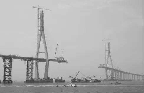
There are case when a two-dimensional study can give fairly good results for instance when the flow around a certain long section of the bridge deck can be regarded as two-dimensional. This is the case when a completed bridge is studied; the flow around the bridge deck is nearly two-dimensional, which means that the flow patterns around different sections are similar. However, if a construction stage is considered, the three-dimensional flow pattern must be taken into account. Such case can be seen in Fig. 2. In this picture the construction of a cable stayed bridge in South Korea is shown. Construction stages are really challenging both from structural dynamics and fluid dynamics point of view.
Manuscript received August 16, 2009. The CFD.hu Ltd., and the Pont-Terv Ltd supported this work.
G. Szabó is with the University of Technology and Economics Budapest, Hungary (corresponding author to provide phone: 0036-30-327-9262; fax: 0036-1-2262096; e-mail: [email protected]).
[image:1.595.306.550.189.336.2]J. Györgyi is with the University of Technology and Economics Budapest, Hungary ([email protected]).
Fig. 1: Tacoma Narrows Bridge flutter (sketch).
At the end of the cantilever (see Fig. 2) the flow field is strongly three-dimensional, which makes the problem really complicated. In these cases the two-dimensional approach might provide unrealistic results. For bridge flutter prediction it is hard to find three-dimensional coupled simulations in literature, but for wing flutter analysis good results can be found in [5]. The main goal in this study is to scrutinize the very complicated three-dimensional response of a bridge deck due to wind loading by using advanced numerical simulation so that assumptions and simplifications should not be needed during the modeling process.
For our purposes an efficient tool was required to handle both the structural behavior and the fluid flow. The target software has to offer coupling abilities between structural dynamics and fluid dynamics. Considering the lack of three-dimensional coupled numerical simulation in literature, a wind tunnel model is to be made in order to have a chance for validation.
Fig. 2: construction of the Incheon bridge in South Korea.
Three-dimensional Fluid-Structure Interaction
Analysis for Bridge Aeroelasticity
[image:1.595.305.549.607.765.2]II. PROBLEM DISCRIPTION
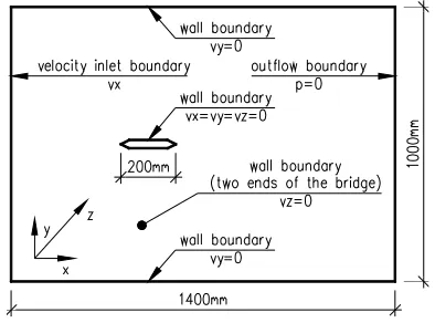
[image:2.595.315.551.47.298.2]Experiences in wind tunnel testing according to [6] and two-dimensional CFD runs [7] were strongly required to start a three-dimensional coupled numerical simulation. The ANSYS 11.0 version was chosen with CSD (Computational Solid Dynamics) and CFD (Computational Fluid Dynamics) tools. By using the MFX multi-field solver involved in the ANSYS, these two physics can be combined in one simulation. As there are measurements for section models only available, a fictive wind tunnel model was considered which is now being constructed. This model is expected to provide enough results to validate the MFX solver of the ANSYS. This wind tunnel model is a two meters long full aeroelastic model, which does not represent a real full-scale bridge, but is really similar to usual wind tunnel models. The bridge is a suspension bridge. The cables are modeled with steel wires, which support the aluminium core beam. On the core beam, balsa segments are fixed, which represent the shape of the bridge. The cross section of our model can be seen in Fig. 3.
Fig. 3: main dimensions of the wind tunnel model.
During the measurement the above detailed model will be mounted in the wind tunnel. The inflow wind velocity is to be varied within a certain range. At a certain wind speed the model is expected to vibrate. The vibration amplitudes should be measured. The wind speed, at which the model starts to oscillate, is the critical wind speed of the flutter instability. The critical wind speed is the target result from the study.
III. COMPUTATIONAL SOLID DYNAMICS The wind tunnel model and its CSD (Computational Solid Dynamics) model have to provide the same dynamic behavior though it is not easy to accomplish. While the wind tunnel model consist of a aluminium core beam bounded with a light material which gives the shape of the bridge, the CSD model is made up by using shell elements, by means of FEM (Finite Element Method). The material properties and the thickness value of the shell elements have to be adjusted in case of the CSD model in order to reach similarity. In the fluid-structure interaction calculation the force-displacement transfer on the boundary of the structure and the fluid flow happens on the bridge deck surface but the cable elements have a role on the structural behavior only. In Fig. 4 the details of the FEM model can be seen. The FEM mesh consists of regular rectangular 4-node shell elements with six degrees of freedom per each node while the cable elements are modeled with link elements without bending capabilities. The surface of the shell must be stiffened with diaphragms at every single cable joints to the bridge deck.
Fig. 4: FEM model details of the bridge.
In the coupled simulation the deformation of the structure is calculated at time steps. The ANSYS uses the Newmark time advancement scheme. In this method the discrete formulation of the structure is required (1), where M, C, and K are the mass, damping, and stiffness matrices respectively while x is the unknown displacement vector, q is the external load vector. The discrete form of (1) can be seen in (2). The solution methodology is as follows; at every single time step the (2) linear equation system is solved for the x displacement vector in the i+1 time step with the ∆t time step size. The extended stiffness matrix and load vector are evaluated in (3) and (4). In (5) and (6) the acceleration and velocity vectors are determined respectively. The solver is unconditionally stable by applying α and β stability parameters. In the simulation the Rayleigh damping was used.
) ( ) ( ) ( )
(t Cx t Kx t q t x
M&& + & + & = (1)
1 1 ˆ
+ + = i
i p x K (2) C t M t K K ∆ + ∆ + = β α β 2 1 ˆ (3)
[
]
∆ − + − + ∆ + − + ∆ + ∆ + = + + i i i i i i i i x t x x t C x t x x t M q p & & & & & & 1 2 1 1 2 1 1 2 1 1 β α β α β α β β (4)[
i i i]
ii x x x t x
t
x& & &&
& − − ∆ − − ∆ = + + 1 2 1 1 1 2 1 β β (5)
[
x x]
x txt
x&i i i &i ∆ &&
[image:2.595.49.290.307.390.2]Before applying the Newmark method, it is highly recommended to perform a dynamic eigenvalue calculation. The results from this simulation are the natural frequencies of the system and the corresponding mode shapes. These dynamic properties are really important to be understood; the behavior of the system due to various load cases can be predicted by studying them.
[image:3.595.57.279.261.754.2]The first four mode shapes of the bridge model can be seen in Fig. 5. The first and the second modes are asymmetrical and symmetrical shapes respectively with pure vertical motion. The third shape belongs to the torsion of the bridge deck. The fourth one shows a horizontal motion of the bridge deck. The natural frequencies are 1.61Hz, 2.45Hz, 6.33Hz, and, 9.55Hz respectively. In the flutter phenomena the torsion mode has the most important role, but according to recent flutter studies, about the first ten shapes have to be included in the simulation.
Fig. 5: the first four mode shapes of the FEM model.
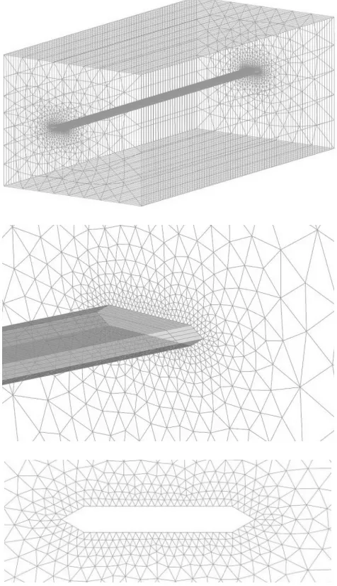
[image:3.595.308.546.345.758.2]IV. COMPUTATIONAL FLUID DYNAMICS Once the CSD model is made, the CFD model is to be built. For the CFD calculations the CFX module of the ANSYS system was used. The software uses the Finite Volume Method for the spatial discretization. This technique requires subdividing the domain of the flow into cells. For the CFD calculations a relatively coarse mesh was made to reduce the computational efforts. The number of cells was around 200.000. The CFD mesh can be seen in Fig. 6. The numerical mesh was made around the bridge contour in two-dimension first. The meshing is finer around the bridge and coarser in the farther reaches of the computational domain. To ensure that, unstructured mesh was used in the plane perpendicular to the bridge axis. This mesh was extruded along the bridge axis providing a structured longitudinal mesh. The computational domain can be seen in Fig. 7. In the vicinity of the bridge contour the velocity and pressure gradients are high, however, considering that the present study is preliminary, the coarse mesh around the bridge contour is acceptable. Naturally precise pressure distribution cannot be expected by this way. Nevertheless, for the CSD calculation rough pressure distribution calculation is enough in this stage of the research, and probably the results are good in order.
Fig. 7: computational domain.
From the CFD simulation the pressure distribution is needed. To obtain that, the Navier-Stokes equation (7) with the continuity equation should be solved.
∂ ∂ + ∂ ∂ + ∂ ∂ + ∂ ∂ − = ∂ ∂ + ∂ ∂ + ∂ ∂ + ∂ ∂ 2 x 2 2 x 2 2 x 2 x x z x y x x x z y x v x ρ 1 g z y x t v v v p v v v v v v v ∂ ∂ + ∂ ∂ + ∂ ∂ + ∂ ∂ − = ∂ ∂ + ∂ ∂ + ∂ ∂ + ∂ ∂ 2 y 2 2 y 2 2 y 2 y y z y y y x y z y x v y ρ 1 g z y x t v v v p v v v v v v v ∂ ∂ + ∂ ∂ + ∂ ∂ + ∂ ∂ − = ∂ ∂ + ∂ ∂ + ∂ ∂ + ∂ ∂ 2 z 2 2 z 2 2 z 2 z z z z y z x z z v y v x v v z ρ 1 g z y x t p v v v v v v v 0 z y x z y x = ∂ ∂ + ∂ ∂ + ∂
∂v v v (7)
Firstly, the N-S equation is averaged in time, which gives the so-called Reynolds stress tensor. This gives six more unknowns therefore closure (turbulence) models have to be applied. In CFD codes there are many turbulence models available but unfortunately none of them is perfect for all kind of flow patterns. In this work the k-ε model was used for its robustness and reliability. The k is the turbulent kinetic energy and ε is the energy dissipation. In CFD applications this one is the most widely used.
V. FLUID-STRUCTURE INTERACTION For the fluid-structure interaction simulation the CSD and the CFD models are necessary. The geometry of them must be conform. The key momentum in the coupled simulation is that the fluid flow induces forces on the bridge deck, which deforms accordingly by using the CSD calculations. The deformations are fed back to the CFD mesh. The time step was set to 0.0008 seconds. The end time was 0.48s, which needed 6 days run time on a four core 2.40 GHz computer with 4.0 GB RAM memories.
The inflow velocity was varied from 5 to 10m/s. From a non-deformed initial state of the bridge, the development of the flutter motion needs much time. Thus, the bridge deck was loaded with a torsion moment for a certain transient time and then it was released, and the free vibration was investigated afterwards. If the amplitudes do not grow, the system could be regarded as stable under these conditions. At the velocities of 5.0 and 7.5 m/s flutter does not occur. At the speed of 10.0 m/s the vibration amplitudes grew from the initial value. This state showed a typical flutter phenomenon.
VI. RESULTS
In Fig. 8 the flow around the deformed bridge deck is shown at the speed of 7.5m/s at different time steps. As the cable elements do not take part in the solid-fluid coupling, they are not shown at all. In the total deformation the torsion of the bridge deck dominates combined with a little vertical displacement. The thin lines on the surface of the bridge show the deformed CFD mesh.
The bridge shape is considered to be streamlined, so great and intensive vortices are not expected to be present nor flow separation from the body. This is why a coarse mesh might be adequate for shapes like this.
[image:4.595.306.546.298.759.2]In case of bridge sections with sharp edges (Fig. 1), however, the flutter phenomenon is accompanied with strong vortices. By using the k-ε or similar turbulence models the accurate modeling of such flow patterns is unlikely. For problems like that, LES (Large Eddy Simulation) turbulence model is offered, which provides accurate results but at an extremely high computational cost.
VII. CHECK OF THE RESULTS
Due to the rather complicated solution introduced above, there is a need to check roughly its reliability. The dynamic loading due to the airflow was strongly simplified for this purpose; for different angles of attack the lift forces and moments can be calculated assuming flat plate theory with the following expressions:
). sin( 2
2 2
γ ρ
π U LB
F = (8)
). sin( 2
2
2 2
γ ρ
π
LB U
M = (9)
In the expressions above ρ is the air density, U is the airflow velocity, L is the section length, and B is the plate width. The simplified aerodynamic forces as a function of the angle of attack (γ) are shown in Fig. 9 for U=7.5m/s wind speed. As it can be seen, in this angle of attack range, the functions are almost linear.
The flow calculation time has been decreased radically by using (8) and (9). To reduce that of the CSD model, it has been simplified as well. This CSD model, made with the ANSYS software, can be seen in Fig. 10. In this model the cable elements were modeled by using simple beams with tension-compression capabilities only while the aluminum core beam and the balsa cross beams are modeled with beam elements. The beam elements have six degrees of freedom per each node. The bridge is fully constrained at both ends. The beam model is able to approximate the behavior of that of the previously introduced more complex model.
-1,20 -0,80 -0,40 0,00 0,40 0,80 1,20
-10 -8 -6 -4 -2 0 2 4 6 8 10
Gamma [degrees]
L
if
t
fo
rc
e
[
N
];
M
o
m
e
n
t
[N
m
]
[image:5.595.289.539.56.287.2]F M
Fig. 9: aerodynamic forces with the flat plate theory.
[image:5.595.55.287.457.596.2]Fig. 10: simplified beam model of the bridge.
Fig. 11: two mode shapes of the bridge model.
In Fig. 11 the mode shapes of the beam model can be seen. Above the first mode represents a heave motion while below the torsion mode is shown. Both shapes are very similar to the corresponding modes of the complex CSD model presented previously (see the first and the third shapes in Fig. 5).
A quasi-static approach can be applied by using (8) and (9). To do so, the dynamic equation of motion of the bridge must be written:
). ( ) ( ) ( )
(
0
t q t Kx t x K t
x M
r
= +
+ &
& &
πω
δ (10)
In (10), M and K are the mass matrix and the stiffness matrix respectively, q is the time dependent load vector, δ and ω0r are the logarithmic decrement and the r-th circular frequency of the bridge. The mode shape values of the beam model (see Fig. 11) can be collected in a V vector. By using the V vector and seeking the solution in the form of x=Vy, (10) yields:
). ( )
( )
( )
(
0
t q V t KVy V t y KV V t
y MV
V T T T
r
T + + =
& &
&
πω
δ (11)
. E MV
VT = (12)
. ... ... 02 02 2
01 r n
T
KV
V = ω ω ω (13)
). ( ) ( ) ( )
( )
( 2
0
0 y t y t v q t f t
t
y T r
r r r r
r
r + ω +ω = =
π δ
& &
& (14)
[image:5.595.58.280.616.759.2]In [8] detailed description can be found to solve (14). The solution methodology is as follows; at every single time step the angle of attack relative to the airflow must be determined and for the next time step the lift force and the moment can be calculated by using (8) and (9). For this calculation a program was written with the Matlab software. This approach neglects the induced flow forces due to the motion of the deck. To take them into account, [9] proposes a solution for a three-dimensional beam model including the aerodynamic derivatives of an arbitrary bridge section.
To calculate the critical wind flutter speed of the bridge model, the inflow velocity was increased step by step, and the free damped oscillation of the structure was recorded as in the case of the coupled CSD-CFD model.
In Fig. 12 the vertical motion of the middle point of the bridge is shown at the wind speed of 5.0m/s with the CSD-CFD and the simplified beam model. As it can be seen, both models show a damped free oscillation after releasing them.
As the CSD-CFD coupled model, the beam model was used with increased wind velocities as well. At the speed of 10.0 m/s it also showed flutter-like condition. This means that for this bridge model the critical wind speed of flutter can be between 5.0 and 10.0 m/s. To find all the instabilities versus the flow velocities, the CSD-CFD simulation should be done at various flow velocities. The problem is that every run requires much time. In addition, the present coarse CFD mesh is not adequate for capturing the vortex shedding for instance. Naturally, considering the results from the two strongly different three-dimensional modeling techniques, perfect coincidences cannot be expected. Nevertheless, the agreement in order is very promising for the future work.
-0,004 -0,003 -0,002 -0,001 0,000 0,001 0,002 0,003 0,004
0,00 0,05 0,10 0,15 0,20 0,25 0,30 0,35 0,40 0,45 0,50
Time [s]
D
is
p
la
c
e
m
e
n
t
[m
]
CSD-CFD BEAM-FLATPLATE
Fig. 12: vertical displacement of the bridge
VIII. CONCLUSION
To conclude, in this paper a three-dimensional coupled CSD-CFD simulation was performed. In an attempt to make a validation in the near future, a fictive full aeroelastic wind tunnel model was considered. The shell model of the bridge was built up on the border of the fluid and the solid domain. At the velocity inlet boundary in CFX, constant velocities were defined, and the free vibrating motion of the bridge deck was studied under airflow. The methodology for finding the critical flutter speed was to apply an inlet velocity increasingly in different runs. When the motion amplitude started growing, the critical velocity was found.
At this stage of the research work the wind tunnel test has not been finished, therefore some kind of approximation was needed to check the results of the complex coupled model. Thus, the critical wind speed was checked with a simplified beam model of the bridge combined with a simple load model of the wind. The guess value of the critical wind speed of the two models was in the same order.
The presented three-dimensional CSD-CFD simulation has strong difficulties, indeed, and cannot be regarded as a solution for three-dimensional flutter prediction at this stage of our research. Nevertheless, in the near future, the aeroelastic wind tunnel model will be made so that the methodology can be validated and become a reliable tool in bridge aeroelasticity as well as in other civil engineering applications.
REFERENCES
[1] Scanlan R. H., Tomko J. J., (1971): Airfoil and bridge deck flutter derivatives. ASCE J. of Eng. Mech. 97, 1717-1737.
[2] Zhiwen Z., Zhaoxiang W., Zhengqing C. (2008): Computational fluid dynamic analyses of flutter characteristics for self-anchored suspension bridges, Front. Archit. Civ. Eng. China 2008, 2(3): 267-273
[3] Theodorsen T., (1935): General theory of aerodynamic instability and the mechanism of flutter. TR 496, NACA.
[4] Larsen A., Walther J. H. (1998): Discrete vortex simulation of flow around five generic bridge deck sections. J. Wind Engng. And Industrial Aerodynamics 77-78, 591-602.
[5] Wang Y., Lin Y. (2008): Combination of CFD and CSD packages for fluid-structure interaction, Journal of Hydrodynamics, 2008, 20(6):756-761
[6] Lajos T., Balczó M., Goricsán I., Kovács T., Régent P.,Sebestyén P. (2006): Prediction of wind load acting on telecommmunication masts #paper A-0206, pp.1-8, IABSE Symposium on Responding to Tomorrow's Challenges in Structural Engineering, Budapest. [7] Györgyi J., Szabó G. (2007): Dynamic calculation of reinforced
concrete chimneys for wind effect using the different codes and analysing the soil-structure interaction, #paper 1371, pp.1-12, ECCOMAS Thematic Conference on Computational Methods in Structural Dynamics and Earthquake Engineering, Rethymno, Crete, Greece.
[8] Bathe K. J., Wilson E. L. (1976): Numerical methods in finite element analysis. Englewood Cliffs, New Jersey: Prentice-Hall, Inc., 528 pp, ISBN 0-13-627190-1
[9] Starossek, U. (1998): Complex notation in flutter analysis, ASCE, Journal of Structural Engineering, Vol. 124, No. 8.