Collapsing of non centered parameterised MCMC algorithms with applications to epidemic models

Collapsing of non-centered parameterised MCMC algorithms

with applications to epidemic models

Peter Neal (Lancaster University) and Fei Xiang (University of Cambridge)

May 17, 2016

Running title: Collapsing of MCMC algorithms

Abstract

Data augmentation is required for the implementation of many MCMC algorithms. The inclusion of augmented data can often lead to conditional distributions from well-known probability distribu-tions for some of the parameters in the model. In such cases, collapsing (integrating out parameters) has been shown to improve the performance of MCMC algorithms. We show how integrating out the infection rate parameter in epidemic models leads to efficient MCMC algorithms for two very different epidemic scenarios, final outcome data from a multitype SIR epidemic and longitudinal data from a spatial SI epidemic. The resulting MCMC algorithms give fresh insight into real life epidemic data sets.

Keywords: Collapsing; measles; non-centred MCMC algorithms; spatial epidemics; stochastic epidemic models.

1

Introduction

A key aim of parametric Bayesian statistics is, given dataxwhich are assumed to arise from a modelM with unknown parametersθ, to obtain the posterior distribution ofθ,π(θ|x). For all, but the simplest of problems this is not analytically tractable and often an MCMC algorithm is used to obtain samples from π(θ|x). Furthermore, the implementation of an MCMC algorithm will often require data augmentation,

y, with the resulting algorithm producing samples fromπ(θ,y|x) with the marginal distributionπ(θ|x) of primary interest. This raises the question of how to construct an efficient MCMC algorithm to obtain samples fromπ(θ,y|x)?

givenφandx,π(λ|φ,y,x) is known. In this case, we can simply integrate outλto leaveπ(φ|x). In Liu (1994) particular focus is placed upon collapsing for the Gibbs sampler but the approach can easily be applied to any MCMC algorithm, whereπ(λ|φ,y,x) is known, see, for example Neal and Roberts (2005) for an epidemic example.

In this paperλis the infection rate of an epidemic model. For a number of epidemic models the augmented data can be chosen independently of λleading to a non-centered parameterisation, Papaspiliopouloset al. (2003). We show how the augmented data can be chosen to give a straightforward to compute likelihood. Then by integrating out not only λ but also a subset of the augmented data we obtain a tractable likelihood which can be utilised within an efficient MCMC algorithm. The generic approach is introduced in Section 2 with the details being model specific. The methodology is illustrated with two distinct epidemic models; final outcome data from a multitype SIR epidemic (Section 3) and longitudinal data from a spatialSI epidemic (Section 4). These highlight the ease with which the collapsing of the MCMC algorithm can be implemented and the significant efficiency gains that it offers. Finally, we briefly summarise the findings of the paper in Section 5.

2

Generic collapsing setup

In this Section we outline the generic collapsing approach taken in this paper. This allows us to highlight the key elements in choosing the data augmentation and implementing the collapsing for epidemic models.

Letθ= (λ,φ) andy= (v,w) denote the parameters of the model and the augmented data, respectively. The parameters and augmented data are each divided into two sets withλand v denoting parameters and augmented data which are to be integrated out andφandwdenoting the remaining parameters and augmented data. Throughout this Section we assume that λis one-dimensional, for ease of exposition and since this is the case in the examples in Sections 3 and 4 and generally likely to be the case in practice. However, the following discussion straightforwardly extends toλ being multidimensional and even in the one-dimensional case the effect on the performance of the MCMC algorithm can be dramatic as we highlight in Section 3.

The joint posterior distribution ofθ andysatisfies

π(θ,y|x) ∝ π(x|y,θ)π(y|θ)π(θ). (2.1)

y= (v,w) is independent ofλ. Thirdly, that the augmented data to be integrated out,vis independent ofφandw. Under these assumptions (2.1) satisfies

π(λ,φ,v,w|x) ∝ π(x|v,w, λ,φ)π(v,w|λ,φ)π(λ,φ)

∝ π(x|v,w, λ,φ)π(w|φ)π(v)π(φ)π(λ). (2.2)

The final assumption that we make regards the form of π(x|v,w, λ,φ), we assume that there exists a deterministic function h(·,·,·,·) such that, ifV andW are drawn from π(v) andπ(w|φ), respectively, h(λ,φ,V,W) gives a realisation ofXfrom the modelMwith parametersθ= (λ,φ). Note that different realisations of the process can be generated by changing some or all ofλ,φ, VandW. In this case

π(x|λ,φ,v,w) = 1_{{h(λ,φ,v,w)=x}}. (2.3) This is a general situation observed in both Sections 3 and 4. The discontinuous density in (2.3) can make constructing an efficient MCMC algorithm difficult, see for example Nealet al.(2012). The integration out ofvandλgives

P(φ,w) =

Z

λ

Z

v

1_{{h(λ,φ,v,W)=x}}π(λ)π(v)dvdλ, (2.4) the probability that, givenφ and w, λand v sampled from π(λ) and π(v), respectively, will result in h(λ,φ,v,w) =x. Note that the inclusion of augmented datavinto the model to then simply integrate it out again may seem unnecessary but it is helpful in understanding the model dynamics and enabling us to exploit (2.3) directly. By constructing an MCMC algorithm based on (2.4) rather than (2.3), we are exploiting a Rao-Blackwellisation, see, for example, Smith and Roberts (1993). Specifically, we are replacing an unbiased, indicator function estimate of the likelihood (E[1_{{h(λ,φ,V,W)=x}}|λ,φ] =π(x|λ,φ)) by an unbiased, probability estimate of the likelihood (E[P(φ,W)|φ] =π(x|φ)). As we shall observe in Section 3 this substantially improves the performance of the MCMC algorithm.

By integrating outλandv, it follows from (2.2) and (2.4) that

π(φ,w|x)∝P(φ,w)π(w|φ)π(φ). (2.5)

Therefore it is straightforward to construct an MCMC algorithm which alternates between updating the parametersφand the augmented dataw. However, we want samples fromπ(λ,φ|x). This can easily be done using a sample (φ,w) fromπ(φ,w|x). Then

π(λ|φ,w,x)∝π(λ)

Z

v

We summarise the generic MCMC algorithm with details being model specific and given in Sections 3 and 4.

MCMC algorithm

i) Proposeφ0 from q_φ(φ,·) and accept the proposed move with probability

π(φ0,w|x)q_φ(φ0,φ) π(φ,w|x)q_φ(φ,φ0) ∧1.

ii) Proposew0 from qw(w,·) and accept the proposed move with probability

π(φ,w0|x)qw(w0,w)

π(φ,w|x)qw(w,w0)

∧1.

iii) Sampleπ(λ|φ,w,x) using (2.6).

iv) Storeθ= (λ,φ) as a sample fromπ(θ|x).

In practice steps (i) and (ii) of the algorithm might comprise multiple steps for updating different sets of parameters and augmented data, respectively.

In the examples considered in Sections 3 and 4,λ represents the infection rate and the integrating out the infection rate allows the MCMC algorithm to move efficiently to effectively determine an appropriate infection rate given the other parameters and the augmented data. In both examples the augmented dataw consists ofω, the order of infection,L, the additional infectious pressure required for successive infections and for the measles example in Section 3 the infectious periodsI. In both cases the datavis a subset of the infectious pressuresL, chosen to ensure that the correct number of infections take place. The other parameters (φ) are model specific, vaccine efficacy in the measles example in Section 3 and spatial and background risk to infection in the spatialSI epidemic in Section 4.

3

Final size epidemic data

involves extending the non-centered parameterisation forSIRepidemic models employed in Neal (2012), Section 3 to multiple types of individuals.

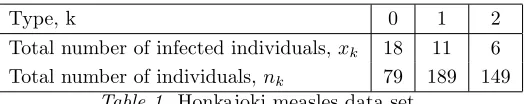
The data consist of how many school pupils were infected in a measles outbreak in Honkajoki, a small rural Finnish municipality in 1989, Paunioet al.(1998). Pupils belong to one of three types, 0, 1 or 2, where a typek (k = 0,1,2) individual has received k doses of measles vaccines. Letxk and nk denote

the total number of infected individuals and the total number of individuals of typek, respectively, with m=x0+x1+x2andN =n0+n1+n2. The data are summarised in Table 1.

Table 1 about here.

A vaccine can affect both an individual’s susceptibility to and infectivity with a disease, Halloran et al. (2010). Given the data, there is insufficient information to model both variable susceptibility and infectivity, see, for example, van Boven et al. (2010), and therefore we assume that the vaccine only affects an individual’s susceptibility to the disease. Therefore the model is as follows. The epidemic is an SIR epidemic in a closed, homogeneously mixing population of sizeN. That is, apart from the initial infective who introduces the disease to the school, nobody is infected from outside the school and we do not model infectious contacts made by pupils with individuals outside of the school. The epidemic is initiated by a single infective with the extension to multiple initial infectives trivial. Whilst infectious, an individual makes infectious contacts at the points of a homogeneous Poisson process with rateλ, with the individual contacted chosen uniformly at random from the population. If the individual contacted by an infective is a susceptible individual of typek, they become infected with probabilityqk, whereq0= 1 and

(q1, q2) are unknown parameters to be estimated. Therefore, fork= 1,2, 1−qk denotes the protective

benefit of being vaccinated ktimes. Infectious contacts with non-susceptible individuals have no affect on the recipient. That is, individuals can be infected at most once. The infectious periods of infected individuals are assumed to be independent and identically distributed according to a random variableI. Final size data contains no temporal information about the epidemic and is invariant to replacing (λ, I) by (cλ, I/c) for any c > 0 (Ball and O’Neill (1999), van Boven et al. (2010), Neal (2012)). Therefore without loss of generality, we take I to have mean 1, so that λ denotes the basic reproduction of the epidemic. We assume U(0,1) priors forq1 andq2 and a Gamma(a, b) prior for λ. (Setting a = 1 and

b= 0 gives an improper uniform prior forλ.)

In order to implement a non-centered parameterisation it is convenient to use a Sellke type construction, Sellke (1983) of the epidemic process, see for example Neal (2012). The construction differs slightly from Neal (2012) in that we have multiple types of individuals. Forj = 0,1,2 andi= 1,2, . . ., letsj,idenote

the total number of susceptibles of type j after the ith _{infection with s}

αi =P 2

j=0sj,iqj/N, the probability that following theith infection, an infectious contact will result in

infection (a contact is with a susceptible and that the contact is successful). We augment the observed datax byω= (ω1, ω2, . . . , ωm),I= (I1, I2, . . . , Im) andL= (L1, L2, . . . , Lm) defined as follows. Letω

denote the order in which individuals are infected withωj =k if thejthindividual infected is of typek.

LetIjdenote the infectious period of thejthindividual. Finally, theLj’s are independent and identically

distributed according toL1∼Exp(1), and their role will be discussed in detail below.

We assume thatωis consistent with the data, that is,xk elements ofωare equal tok(k= 0,1,2). Then

π(ω|q) =

m

Y

i=1

sωi,i−1qωi

P2

k=0sk,i−1qk

, (3.1)

where q0 = 1. Thus the order ω explicitly depends on the parametersq. Given thati infections have

taken placeLi/(αiλ) denotes the additional infectious pressure (units of infection) needed to ensure that

the (i+ 1)st _{individual is infected. This is consistent with infectives making infectious contacts at rateλ}

with success probability αi. Thus, givenω, q,LandI, the epidemic infectsm individuals of typesx, if

for all 1≤k≤m−1,

1 λ k X i=1 Li αi ≤ k X i=1

Ii, (3.2)

and 1 λ m X i=1 Li αi > m X i=1

Ii. (3.3)

Leth(λ,q,ω,L,I) denote the epidemic process generated by the firstminfections. Then ifωis consistent with the data and (3.2) and (3.3) are satisfied, we have that h(λ,q,ω,L,I) =x. We can construct an MCMC algorithm which moves around the joint space of (λ,q,ω,L,I) but we collapse the algorithm by integrate outλand Lm. That is, in the notation of Section 2, φ=q,w = (ω,L1:m−1,I) and v=Lm,

where L1:m−1 = (L1, L2, . . . , Lm−1). By integrating out Lm, a simple conditional distribution for λ,

λ|ω,q,L1:m−1,I,x, exists. From (3.2) and (3.3), we require that

Hm= max 1≤k≤m−1

Pk

i=1Li/αi

Pk

i=1Ii

≤λ <

Pm

i=1Li/αi

Pm

i=1Ii

. (3.4)

Thusλ > HmandLm> αm{λP m

i=1Ii−P m−1

i=1 Li/αi}=Jm, say, gives

P(q,ω,L1:m−1,I|x) ∝

Z ∞

0

Z ∞

0

π(x|λ,q,ω,L,I)π(λ)π(q)π(ω|q)π(L)π(I)dLmdλ

∝

Z ∞

Hm

Z ∞

Jm

exp(−Lm)dLm

λa−1

Γ(a)exp(−λb)dλπ(ω|q)π(L1:m−1)π(I)

= exp αm m−1

X

i=1

Li/αi

!

π(ω|q)π(L1:m−1)π(I)

×

Z ∞

Hm

exp −λαm m

X

i=1

Ii

!

λa−1

The integral on the righthand side of (3.5) isP(Z > Hm)/(b+αmP m

i=1Ii)a, whereZ ∼Gamma(a, b+

αmP m

i=1Ii). Thus if a∈N, corresponding to an Erlang prior (Gamma distribution with integer shape

parameter) onλ, it follows from (3.5) that

P(q,ω,L1:m−1,I|x) =

(a−1

X

k=0

(b+αmP m

i=1Ii)k−a

k!

)

π(ω|q)π(L1:m−1)π(I)

×exp −αm

(

Hm m

X

i=1

Ii− m−1

X

i=1

Li/αi

)!

. (3.6)

We are now in position to describe a collapsed MCMC algorithm based upon (3.5) for obtaining samples from π(λ,q|x). The acceptance probability for each step is straightforward to compute using (3.5) and (3.1). Below we describe the steps per iteration with (λ,q) stored at the end of each iteration.

MCMC algorithm

i) Update (q1, q2) using random walk Metropolis. We proposeqk0 ∼N(qk, σq2) (k= 1,2), with reflection

at the boundaries 0 and 1 to ensure that 0≤q0₁, q0₂≤1.

ii) Update in turn the augmented dataw= (ω,L1:m−1,I) as follows

(a) Updateω using an independence sampler withω0 _{sampled uniformly at random from the set}

of possible orderings consistent with the data.

(b) UpdateL1:m−1 by proposing to update a random subsetP of the thresholds, where|P|=p.

Ifi∈ P, drawL0_i∼Exp(1), otherwise set L0_i=Li.

(c) UpdateIby proposing to update a random subsetRof the infection periods, where|R|=r. Ifi∈ R, drawI_i0∼I, otherwise setI_i0=Ii.

iii) Draw λ|ω,q,L1:m−1,I,x from its conditional distribution, which is Gamma(a, b+αmP m i=1Ii)

conditioned to be greater than Hm. If a = 1, we can exploit the memoryless property of the

exponential random variable to give

λ|ω,q,L1:m−1,I,x∼Hm+ Exp b+αm m

X

i=1

Ii

!

. (3.7)

iv) Storeθ= (λ,q) as a sample fromπ(θ|x).

We briefly comment upon the algorithm for the Honkajoki data. For updatingq, we want an acceptance rate of approximately 35% to optimise the random walk Metropolis. This is achieved by choosingσq =

Xiang and Neal (2014). The independence sampler for ω has a high acceptance rate of 90%, which shows that the order of infection is largely irrelevant. If the data are such that the order ofω is more important an updating scheme along the lines of that used in Section 4 could alternatively be used. For updatingL1:m−1, we choosep= 15, which results in an acceptance rate of 33%. There is a compromise

here as increasingpdecreases the acceptance rate and maximiseptimes the acceptance rate gives close to optimal behaviour, see Xiang and Neal (2014). We choose π(λ) ∝ 1 (λ > 0) corresponding to an improper Gamma(1,0) prior. Finally, we consider three scenarios for I; I ≡1, I ∼Gamma(2,2) and I ∼ Gamma(exp(γ),exp(γ)) with γ unknown. Except in the case where I ≡ 1, we updated r = 15 infection times together at each iteration. In the case of unknown γ we assigned an Exp(1) prior (this ensures that the shape parameter on the Gamma distribution is greater than or equal to 1) and added a random walk step to the MCMC algorithm to updateγwith proposal standard deviation 1.

For all three scenarios the algorithm was run for 110000 iterations with the first 10000 iterations discarded as burn-in. The initial values forq,ωandL1:m−1were drawn from the prior onq, a random permutation

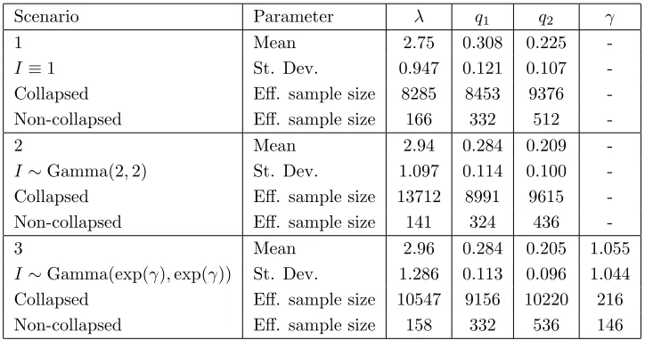
of the m infections and Exp(1), respectively. The initial values for Iare drawn from the appropriate distribution withγ = 1 in the third scenario. The burn-in is excessive with convergence appearing to be almost instantaneous, except for γ. Autocorrelation function plots show that for all the parameters, exceptγ, the correlation is decaying rapidly and is approximately 0 by lag-30. The estimated posterior means, standard deviations and effective sample sizes for (λ,q, γ) are given in Table 2. The poor mixing in γ is due to the lack of information in the final size data about the infectious period distribution, highlighted by the variability inγ and the similar parameter estimates for all three scenarios withI≡1 corresponding to the limit asγ→ ∞ofI∼Gamma(exp(γ),exp(γ)).

Table 2 about here.

For comparison we ran the corresponding MCMC algorithms withoutλandLmintegrated out for 110000

iterations with the first 10000 iterations discarded as burn-in. We initialised with λ= 3 and simulated

q, ω, L andIuntil we obtained an epidemic consistent with the data. The modifications to the above algorithm are thatL is updated in place ofL1:m−1andλdrawn uniformly from

max

1≤k≤m−1

( k

X

i=1

Li

αi

/

k

X

i=1

Ii

)

,

m

X

i=1

Li

αi

/

m

X

i=1

Ii

!

,

which ensures that (3.2) and (3.3) are satisfied. To optimise performance we setσq = 0.05, p= 5 and

r= 5. The estimated posterior means and standard deviations are similar to those reported in Table 2 for the collapsed MCMC algorithm but the mixing is far worse. The estimated effective sample sizes forq1,

with the exception ofγ are in all cases at least 18 times higher for the corresponding collapsed MCMC algorithm and since both the collapsed and non-collapsed MCMC algorithms have virtually identical running times this represents a very significant improvement. The similar performance in the mixing of γin the algorithms is due to the updating ofγonly depending onIand thus is largely unaffected by the inclusion of collapsing.

The choice of an improper Gamma(1,0) prior in the above analysis makes implementing the MCMC algo-rithm particularly straightforward as the first term on the right hand side of (3.6) is simply 1/(αmP

m i=1Ii)

and (3.7) can be exploited to sampleλ. For an Erlang prior distribution, Gamma(a, b) witha∈N, onλ

we can still use (3.6) and sample λfrom a truncated Gamma distribution. This involves minor adjust-ments to the code with very similar results in terms of mixing but with the code taking between 5−10% and 10−15% longer to run with Gamma(2,2) and Gamma(10,10) priors, respectively, onλ.

Finally, in van Bovenet al. (2010) there are other measles data sets which the above MCMC algorithm can be applied to. Moreover, there are data from a measles outbreak from a school in Duisburg, Germany with missing vaccination status for approximately 30% of the population. Details of how to extend the MCMC algorithm to incorporate missing information and the corresponding analysis are given in the supplementary material.

4

Spatial epidemic

highlight the differences and advantages of this approach to that taken in Brown et al. (2014) where estimation of both the spatial spread of the disease and the infection rate is performed. Finally, we employ the new MCMC algorithm to the CTV data, Gibson (1997a) and the spread of SCYLV, Daugrois

et al.(2011), Brownet al. (2014).

Letx,y∈ Ldenote the location of two individuals on a subset ofR2with typicallyLbeing a lattice. Once

individualxis infected it makes infectious contacts with individualyat the points of an inhomogeneous Poisson point process with ratek(t)Fα(x−y), wherek(t) represents an underlying infection rate

(non-negative and possibly time varying) and Fα(·) is a non-negative function (parameterised by α) which

characterises the force of infection fromxandy. Throughout this paper, and in line with previous work, the force of infection between two individuals will depend upon their Euclidean distance andFα(·) will be

a monotonically decreasing function of distance. If individualy is susceptible when individualxmakes infectious contact it becomes infected (and immediately infectious), otherwise the infectious contact has no affect on individualyas it is already infectious. We follow Brownet al.(2014), by assuming thatk(t) is constant (k(t) =λfor allt). (Note that Brownet al.(2014) usesβ rather thanλfor the infection rate.) The extension to piecewise constant infection rates with change points corresponding to the observation times is trivial. Finally, it is commonplace, see, Gibson (1997b) and Brownet al.(2014), to assume that there is an external background risk to infection,k(t)r. Thus ifI denotes the set of location of infectives at timest, the infectious exposure that an individualyis subjected to at timetisλ{r+P

x∈IFα(x−y)}.

The observed data are assumed to be snapshots of theS →I epidemic at a discrete set of time points. Lett0(= 0)< t1< . . . < tmdenote times at which the infectious status of all individuals are known. For

i= 0,1, . . . , m, let Si andIi denote the set of susceptible and infected individuals, respectively at time

point ti. Fori = 1,2, . . . , m, let Wi =Ii\Ii−1, the set of individuals infected between time points ti−1

and ti with ni =|Wi|. In Gibson (1997a), m= 1 and the two time points correspond to dates a year

apart. In Brownet al. (2014),m = 6 with t= (0,6,10,14,19,23,30) and time units of a week. (Note that in this casetshould be (0,6,11,15,19,23,30), see Daugroiset al. (2011).)

In order to construct a tractable likelihood we need to use data augmentation. We begin by following Gibson (1997a) by specifying the order in which infections occur in a given interval. Letyω(i,j) denote

thejth_{individual infected in thei}th_{time interval. LetQ}

i,j denote the length of time from the (j−1)st

infection in time intervaliuntil thejth _{infection, where the time of the 0}th_{infection is taken to bet} i−1

infectives and susceptibles, respectively, after thej−1st infection in time intervali,

Qi,j ∼ Exp



λ X

y∈Si,j−1

 



r+ X

x∈Ii,j−1

Fα(x−y)

     =    λ X

y∈Si,j−1

 



r+ X

x∈Ii,j−1

Fα(x−y)

      −1 Exp(1)

= {λhi,j(α, r,ω)}−1Li,j, say, (4.1)

where ω and ωi _{denote the total set of infection orderings and the total set of infection orderings in}

time intervali, respectively. We will primarily useLi,j rather thanQi,j in the data augmentation since

a prioriLi,j ∼Exp(1), a non-centered parameterisation. Note thatLi,j has the same distribution toLi

in Section 3 and plays the same role in defining the additional infectious pressure required for the next infection. LetLi _{= (L}

i,1, . . . , Li,ni+1) and L = (L

1_{, . . . ,L}m_{). Then exploiting the independence of the}

epidemic process between different time intervals,

π(I,ω,L|r, α, λ) =

m

Y

i=1

π(Ii|ωi,Li, α, λ)

= m Y i=1   

1{Ui}

ni

Y

j=1

r+P

x∈Ii,j−1Fα(x−yω(i,j))

hi,j(α, r,ω)

!ni+1

Y

j=1

exp(−Li,j)

 



, (4.2)

whereUi denotes the event thatni infections take place in intervaliwith

1{Ui}= 1n Pni

j=1Li,j/(λhi,j(α,r,ω))≤ti−ti−1<Pnij=1+1Li,j/(λhi,j(α,r,ω))

o. (4.3)

Note that theni+ 1stinfection after timeticorresponds to the first infection after timeti+1. We include

both Li,ni+1 and Li+1,1 in the likelihood, as we explicitly use Li+1,1 for the time of the first infection

in interval i+ 1 and integrate out Li,ni+1 to ensure that ni infections occur in interval i. Moreover,

the condition (4.3) mirrors the conditions for fixing the size of the measles epidemic, (3.2) and (3.3), in that we require λ to be large enough, so thatni infections occur in interval i, but also to be small

enough that no more infections take place. Thus mirroring Section 3 we seek to integrate out λ and (L1,n1+1, . . . , Lm,nm+1), the additional infectious pressure to the next infection.

From (4.2), we have that

π(ω,L, r, α, λ|I) ∝ π(I,ω,L|r, α, λ)π(r)π(α)π(λ). (4.4)

We proceed by integrating out λand (L1,n1+1, . . . , Lm,nm+1) before outlining the MCMC algorithm for

sampled at each iteration as an add-on to the MCMC algorithm of Gibson (1997a). This corresponds to fully integrating outLin the updating ofr, αandω. Details of the generalisation tom >1 and a Gamma prior onλ, where full integration out ofLis not possible are given in the supplementary material.

Consider the casem= 1 andπ(λ)∝1 (λ >0). Then letting ˇL1_{= (L}

1,1, . . . , L1,n1), we have that

π(ω,Lˇ1, r, α|I) ∝

Z

λ

Z

L1,n_{1 +1}

π(I,ω,L|r, α, λ)π(r)π(α)π(λ)dL1,n1+1dλ

=

n1

Y

j=1

r+P

x∈Ii,j−1Fα(x−yω(i,j))

hi,j(α, r,ω)

! n1

Y

j=1

exp(−Li,j)π(r)π(α)

×

Z

λ

Z

L1,n_{1 +1}

exp(−L1,n1+1)1{U1}dL1,n1+1dλ

= K

Z

λ

Z

L1,n1 +1

exp(−L1,n1+1)1{U1}dL1,n1+1dλ, say. (4.5)

Givenλ, for 1{U1}to be equal to 1, we require that

L1,(n1+1)> λh1,n+1(α, r,ω)



t1−

1 λ n1 X j=1 1 h1,j(α, r,ω)

L1,j



>0. (4.6)

Therefore it follows from (4.5) with

C=



λh1,n+1(α, r,ω)



t1−

1 λ n1 X j=1 1 hi,j(α, r,ω)

L1,j  ,∞   that

π(ω,Lˇ1, r, α|I)

∝ K

Z

λ

1_{λ>Pn1 j=1

1

h_1,j(α,r,ω)L1,j/t1}

Z

L1,n1 +1∈C

exp(−L1,n1+1)dL1,n1+1dλ

= K

Z

λ

1_{λ>Pn1

j=1h1,j(α,r,1 ω)L1,j/t1}

exp(−λh1,t+1(α, r,ω)t1)

×exp



h1,n1+1

n1

X

j=1

1 h1,j(α, r,ω)

L1,j



dλ

= Kexp



h1,n1+1(α, r,ω)

n1

X

j=1

1 h1,j(α, r,ω)

L1,j   × − 1

h1,n1+1(α, r,ω)t

exp (−λh1,n1+1(α, r,ω)t1)

∞

Pn1

j=1h1,j(α,r,1 ω)L1,j/t1

=

n1

Y

j=1

r+P

x∈I1,j−1Fα(x−yω(1,j))

h1,j(α, r,ω)

! n1

Y

j=1

exp(−L1,j)π(r)π(α)

1

h1,n1+1(α, r,ω)t1

.

(4.7)

Note that it follows from the third line of (4.7) that

λ|ω,Lˇ1, r, α,I ∼

n1

X

j=1

L1,j

h1,j(α, r,ω)t1

Furthermore in (4.7), the only term involving ˇL1_isQn1

j=1exp(−L1,j). Therefore integrating out ˇL1yields,

π(ω, r, α|I) ∝

n1

Y

j=1

r+P

x∈I1,j−1Fα(x−yω(1,j))

h1,j(α, r,ω)

!

π(r)π(α)

× 1

h1,n1+1(α, r,ω)

. (4.9)

We observe that (4.9) differs slightly to π(ω, r, α|I) given in Gibson (1997a) including the final term 1/h1,n1+1(α, r,ω). The difference is due to the slightly different scenarios considered. In Gibson (1997a),

the posterior is derived based upon, from time 0 the nextn1 infections being the set of individuals W1,

regardless of the time taken. Since we are explicitly taking into account time, as well as requiring the next n1 infections to be the set of individuals W1, we also require that no more infections take place.

Ignoring this leads to a slight bias in the estimation ofαandr. The largerh1,n1+1(α, r,ω) is, the smaller

the range ofλvalues (combined withL1_{) which are consistent with exactlyn}

1infections taking place in

the time interval.

For m ≥ 1, we can update ω efficiently using a scheme based upon Gibson (1997a). Specifically, we propose to switch (ωi,j, ωi,j+1) in a systematic manner. The key observation is that the changes in the

likelihood involved with switching (ωi,j, ωi,j+1), only depends upon who has been infected prior to the

jth_{infection in time intervaliand not the order in which they were infected. Furthermore, the order of}

infection of individuals (ωi,j, ωi,j+1) has no effect on any subsequent infections. Therefore for alli, we

can consider the switching the orders of infected pairs

(ωi,1, ωi,2),(ωi,3, ωi,4), . . . ,(ωi,2mi−1, ωi,2mi), (4.10)

in parallel, wheremi is the largest integer such that 2mi≤ni. Also for alli, the switches

(ωi,2, ωi,3),(ωi,4, ωi,5), . . . ,(ωi,2ki, ωi,2ki+1) (4.11)

can be considered in parallel, whereki is the largest integer such that 2ki+ 1≤ni.

We are now in position to outline an iteration of the MCMC algorithm form= 1 with (r, α, λ) stored at the end of each iteration. The extension tom >1 is given in the supplementary material.

MCMC algorithm

i) Update (r, α) using random walk Metropolis with a bivariate Gaussian proposal. Use (4.9) to compute the acceptance probability.

(a) For l = 1,2, . . . , m1, propose to switch the order of infection for (ω1,2l−1, ω1,2l), sequentially

or preferably in parallel.

(b) Forl= 1,2, . . . , k1, propose to switch the order of infection for (ω1,2l, ω1,2l+1), sequentially or

preferably in parallel.

iii) Sampleλ. Simply draw a new set ˇL1 _{and then sampleλ|ω,L}ˇ1_{, r, α,I from its conditional}

distribu-tion given by (4.8).

iv) Store (λ, r, α) as a sample fromπ(θ|x).

Finally, before implementing the MCMC algorithm, we compare our approach to Brown et al. (2014), where estimation ofµ=λr, αand λ(=β) is performed. In Brown et al. (2014), the infection times τ of the plants are imputed rather than the order of infection and the inter-infection time intervals. Note that τ can easily be obtained from λ, ω and ˇL and visa-versa. The main disadvantage of the MCMC algorithm of Brown et al. (2014) is that updating an element of τ has an effect on many components of the likelihood (all subsequent infection times), whereas the update ω can, as noted above, be done efficiently and quickly by switching the orders of infection.

We now employ the MCMC algorithm to estimate the parameters for the CTV data and the SCYLV data. The CTV data introduced in Marcuset al.(1984) and analysed in Gibson (1997a) is used to illustrate the methodology with m= 1, whilst the main emphasis is on the longitudinal analysis of the SCYLV data experiment in Daugroiset al.(2011), analysed in Brownet al.(2014). The CTV data consist of the locations of infected trees in a citrus orchard at two time points, 1 year apart. There are 131 infected trees discovered at the first time point, 1981 with a further 45 trees infected by the second time point, 1982. In Gibson (1997a), there is assumed to be no background infection (r = 0) and two choices of Fα(x−y) are considered; (a) exp(−α|y−x|) and (b)|y−x|−2αwithαestimated on the basis of the 45

infections between the two observed time points. For both cases we estimatedαandλbased on 50,000 iterations following a burn-in of 2,000 iterations. The posterior means (standard deviations) of αand λ are, for case (a), 0.269 (0.0678) and 0.168 (0.113), respectively, and for case (b), 1.32 (0.158) and 3.05 (2.54), respectively. The estimates forαare consistent with those presented in Gibson (1997a) where a discrete set of αvalues rather than the continuous model presented here are used. It should be noted that the non-collapsed MCMC algorithm was not a practical alternative to the collapsed algorithm as the key condition (4.3) was often violated, and proposed moves rejected, for all but very small moves in θ= (λ, r, α) andL, even with longer runs of 106 _iterations.

in the forthcoming year. However, we use knowledge ofλto estimate the time of the introductory case of CTV into the orchard. We follow Gibson (1997a) by modelling the first 176 infectious cases, assuming that there is a single introductory case, whose location is unknown but is one of the 131 locations infected before the end of 1981. The parameterαis estimated based on the full data, whereas the 45 infections occurring between the two observation points allow us to estimateλ. Then fori= 2,3, . . . ,131, we can simulate the length of time,X0

i, between the (i−1)standithinfection withXi0∼Exp(λ

P

x∈I0,i−1

P

y∈S0,i−1Fα(x− y)). Thus T0 = P

131 i=2X

0

i represents an estimate of the time of the introductory case prior to the first

time point (1981). Using Fα(x−y) = exp(−α|y−x|), the posterior means (standard deviations) of α

and λare 0.1071 (0.0141) and 0.0192 (0.0061), respectively. The estimate ofαis again consistent with corresponding analysis in Gibson (1997a). However, unlike Gibson (1997a), we can estimateT0 which is

found to have a posterior mean of 15.3 years with a standard deviation of 4.5 years.

In Brownet al.(2014) trial B from Daugroiset al.(2011) is analysed. Specifically, Daugroiset al.(2011) details four trials of the spread of SCYLV in trial plantations which are initially disease-free. The SCYLV is transmitted from plant to plant via aphids. The infectious status of all 1742 plants in trial B were recorded at weeks 0,6,11,15,19,23 and 30. As noted above this differs slightly from Brown et al.(2014) but this difference has very little effect on parameter estimates. We follow Brownet al.(2014) in taking Fα(x−y) =_2πα12exp(−|x−y|

2_/(2α2_{)), a Gaussian transmission kernel proposed in Brownet al.(2014) to}

estimates based on the full data set as opposed to taking it as a single time interval with a clear loss of information from not taking into account the temporal spread of the disease.

There are a couple of observations to make about the analysis of the data. Firstly, in the switching step for updatingωthe proportion of moves accepted was over 99% for all positions over both data sets. This corresponds to their being little information in the data concerning the order of infection and is consistent with the plots of the density of infection times in the first and last intervals presented in Brownet al.

(2014), Figure 3. We applied the MCMC algorithm to a small simulated data set presented in Gibson (1997a), Figure 3 with one initial infective and nine subsequent infections. Even in this case with clear chains of infection the acceptance rates for all positions in updatingωwere over 75%, increasing to 92% for the final position. This all suggests that, if a reasonable initial choice ofωis made, decent parameter estimates can be obtained even ifωis kept fixed (not updated). We proposed a fixed configuration forω chosen usingr= 0.1 andα= 1.0 and then estimated the parametersµ, αand λusing a MCMC run of 110,000 iterations with the first 10,000 iterations discarded as burn-in andωkept fixed. The algorithm ran approximately four times as fast without the update of theωand we obtained 0.0026 (0.00035), 1.17 (0.091) and 0.116 (0.0060) for the posterior means and standard deviations of the parametersµ(=rλ),α andλ, respectively. Thus we obtain a reasonable approximation of the posterior distribution in this case. Similar results were obtained starting fromr= 0.001 andα= 2.0, details along with plots are presented in the supplementary material. Secondly, the algorithm performs very well for a single time interval with mixing worsening as the number of time intervals increases. The main reason for the algorithm performing particularly well for a single time interval is the ability to full integrate out ˇL as evidenced by the considerably larger proposal standard deviations used for a single time interval as opposed to that used for the full data.

5

Conclusions

Poisson processes gives great flexibility in modelling the infectious process and in particular, leads to the exponential tolerances, L exploited in both examples in this paper. Therefore the data augmentations and collapsing developed in this paper should be applicable to a wider class of epidemic models than the two presented here.

More generally, it is the Markov property of the Poisson process which is particularly useful here. In Neal (2014) a simple reparameterisation of Markov processes is exploited to allow coupled simulations of a Markov process. Specifically, if θ = (θ1, θ2, . . . , θp) represent rate parameters of a Markov process,

then we can reparameterise by settingλ=θpandφ= (θ1/θp, θ2/θp, . . . , θp−1/θp). Thus the components

of φ are the relative rates of parameters θ to λ = θp. For a Markov process it is φ and the state of

the system which determine the probability that a given transition takes place, whereas λ determines the inter-arrival time between events. This is similar to the epidemic examples studied here, in that, the infection rateλdetermines the additional infectious pressure required for the next infection and the other parameters and state of the population that determine who gets infected.

A simple example of a Markov process is theSIS epidemic model. Suppose that we have a population of size n and let Y(t) denote the total number of infectives at time t. Since individuals can only be susceptible or infectious,Y(t) defines the state of the system withn−Y(t) being the number the number of susceptibles. Let infectious individuals make infectious contacts at the points of a homogeneous Poisson point process with rateβ and recover at rateγ (exponentially distributed infectious periods with mean 1/γ). Letλ=γ and φ=β/γ. Then at time t, the time until the next event (infection or recovery) is Exp(βY(t)(n−Y(t))/n+γY(t)) = Exp(φY(t)(n−Y(t))/n+Y(t))/λand the probability that the next event is an infection is

βY(t)(n−Y(t))/n βY(t)(n−Y(t))/n+γY(t) =

φ(n−Y(t))/n

φ(n−Y(t))/n+ 1. (5.1)

infection time at a time leading to slow exploration of the space of the number of unobserved infectives.

Acknowledgements

This work was supported by EPSRC grant, EP/J008443/1. We would like to thank Patrick Brown and Jean Heinrich Daugrois for providing access to and guidance on the sugarcane yellow leaf virus data set. We would like to thank two anonymous referees’ and an associate editor for their comments which have assisted in revising the paper.

Supporting information. Additional supporting information may be found in the online version of this article at the publishers website.

References

Ball, F. and O’Neill, P. (1999) The distribution of general final state random variables for stochastic epidemic models.J. Appl. Probab.,36, 473–491.

van Boven, M., Kretzschmar, M., Wallinga, J., O’Neill, P.D., Wichmann, O. and Hahn´e, S. (2010) Esti-mation of measles vaccine efficacy and critical vaccination coverage in a highly vaccinated population. Journal of the Royal Society Interface,7, 1537–1544.

Brown, P.E, Chimard, F., Remorov, A., Rosenthal, J.S. and Wang, X. (2014) Statistical Inference and Computational Efficiency for Spatial Infectious-Disease Models with Plantation Data.J. R. Stat. Soc. Ser. C. Appl. Stat.63, 467–482.

Daugrois, J.H., Edon-Jock, C., Bonoto, S., Vaillant, J. and Rott, P. (2011) Spread of Sugarcane yellow leaf virus in initially disease-free sugarcane is linked to rainfall and host resistance in the humid tropical environment of Guadeloupe.European Journal of Plant Pathology129, 71-80.

Gibson, G.J. (1997a) Markov Chain Monte Carlo Methods for Fitting Spatiotemporal Stochastic Models in Plant Epidemiology.J. R. Stat. Soc. Ser. C. Appl. Stat. 46, 215–233.

Gibson, G.J. (1997b) Investigating mechanisms of spatiotemporal epidemic spread using stochastic mod-els.American Phytopathological Society87, 139–146.

Halloran, M. E., Longini, I. M. and Struchiner, C. J. (2010) Design and analysis of vaccine studies.

Jewell, C.P., Kypraios, T., Neal, P.J. and Roberts, G.O. (2009) Bayesian Analysis for Emerging Infectious Diseases.Bayesian Analysis4, 465–496.

Liu, J.S. (1994) The collased Gibbs sampler in Bayesian computations with applications to a gene regu-lation problem.J. Amer. Statist. Assoc.89, 958–966.

Marcus, R., Svetlana, F., Talpaz, H., Salomon, R. and Bar-Joseph, M. (1984) On the spatial distribution of citrus tristeza virus disease.Phytoparasitica12, 45–52.

Neal, P. (2012) Efficient likelihood-free Bayesian Computation for household epidemics.Statist. Comput.,

22, 1239–1256.

Neal, P. (2014) Simulation based sequential Monte Carlo methods for discretely observed Markov pro-cesses. arXiv:1404.4185

Neal, P.J. and Huang, C.L.T. (2015) Forward simulation MCMC with applications to stochastic epidemic models.Scand. J. Statist.42, 378–396.

Neal, P.J. and Roberts, G.O. (2005) A case study in non-centering for data augmentation: Stochastic epidemics.Statist. Comput. 15, 315–327.

Neal, P.J., Roberts, G.O. and Yuen, W.K. (2012) Optimal Scaling of Random Walk Metropolisalgorithms with discontinuous target densities.Ann. Appl. Probab.22, 1880–1927

O’Neill, P.D. and Roberts, G.O. (1999). Bayesian inference for partially observed stochastic epidemics.

J. Roy. Statist. Soc. Ser. A162, 121–129.

Papaspiliopoulos, O., Roberts, G.O. and Sk¨old, M. (2003) Non-centered parameterisations for hierarchical models and data augmentation. Bayesian Statistics 7 (J.M. Bernardo, M.J. Bayarri, J.O. Berger, A.P. Dawid, D. Heckerman, A.F.M. Smith and M. West, eds.) Oxford University Press, 307–326.

Paunio, M., Peltola, H., Valle, M., Davidkin, I., Virtanen, M. and Heinonen, O. (1998) Explosive school-based measles outbreak: Intense exposure may have resulted in high risk, even among revaccinees

American Journal of Epidemiology,148, 1103–1110.

Sellke, T. (1983) On the asymptotic distribution of the size of a stochastic epidemic.J. Appl. Probab.20, 390–394.

Streftaris, G. and Gibson, G.J. (2012) Nonexponential tolerance to infection in epidemic systems -modeling, inference and assessment.Biostatistics13, 580–593.

Tanaka, M. M., Francis, A. R., Luciani, F. and Sisson, S. A. (2006) Using approximate Bayesian compu-tation to estimate tuberculosis transmission parameters from genotype data.Genetics173, 1511–1520.

Tavar´e, S., Balding, D.J., Griffiths, R.C. and Donnelly, P. (1997) Inferring coalescence times from DNA sequence data.Genetics,145, 505–518.

Xiang, F. and Neal, P. (2014) Efficient MCMC for temporal epidemics via parameter reduction.Comput. Statist. Data Anal.80, 240–250.

Corresponding author’s address: Fylde College

Lancaster University Lancaster

LA1 4YF United Kingdom

Type, k 0 1 2 Total number of infected individuals,xk 18 11 6

Total number of individuals,nk 79 189 149

Scenario Parameter λ q1 q2 γ

1 Mean 2.75 0.308 0.225

-I≡1 St. Dev. 0.947 0.121 0.107

-Collapsed Eff. sample size 8285 8453 9376

-Non-collapsed Eff. sample size 166 332 512

-2 Mean 2.94 0.284 0.209

-I∼Gamma(2,2) St. Dev. 1.097 0.114 0.100

-Collapsed Eff. sample size 13712 8991 9615

-Non-collapsed Eff. sample size 141 324 436

-3 Mean 2.96 0.284 0.205 1.055

I∼Gamma(exp(γ),exp(γ)) St. Dev. 1.286 0.113 0.096 1.044

Collapsed Eff. sample size 10547 9156 10220 216

Non-collapsed Eff. sample size 158 332 536 146

Table 2. Estimated posterior means, standard deviations and effective sample size (collapsed and non-collapsed)λ,qandγ, for the three scenarios 1)I≡1; 2)I∼Gamma(2,2) and 3)