A Poisson process reparameterisation for Bayesian inference for extremes

A Poisson process reparameterisation for Bayesian inference for

extremes

Paul Sharkey and Jonathan A. Tawn

Email: [email protected],[email protected]

STOR-i Centre for Doctoral Training, Department of Mathematics and Statistics, Lancaster

University, Lancaster, LA1 4YF, U.K.

Abstract

A common approach to modelling extreme values is to consider the excesses above a high threshold as realisations of a non-homogeneous Poisson process. While this method offers the advantage of modelling using threshold-invariant extreme value parameters, the dependence between these parameters makes estimation more difficult. We present a novel approach for Bayesian estimation of the Poisson process model parameters by reparameterising in terms of a tuning parameterm. This paper presents a method for choosing the optimal value ofmthat near-orthogonalises the parameters, which is achieved by minimising the correlation between the asymptotic posterior distribution of the parameters. This choice ofm ensures more rapid convergence and efficient sampling from the joint posterior distribution using Markov Chain Monte Carlo methods. Samples from the parameterisation of interest are then obtained by a simple transform. Results are presented in the cases of identically and non-identically distributed models for extreme rainfall in Cumbria, UK.

Keywords: Poisson processes, Extreme value theory, Bayesian inference, Reparameterisation,

Covariate modelling.

1

A Poisson Process model for Extremes

The aim of extreme value analysis is to model rare occurrences of an observed process to extrapolate

to give estimates of the probabilities of unobserved levels. In this way, one can make predictions

of future extreme behaviour by estimating the behaviour of the process using an asymptotically

justified limit model. LetX1, X2, . . . , Xnbe a series of independent and identically distributed (iid)

random variables with common distribution function F. Defining Mn = max{X1, X2, . . . , Xn}, if

there exists sequences of normalising constants an>0 andbn such that:

Pr

Mn−bn

an

≤x

where G is non-degenerate, then G follows a generalised extreme value (GEV) distribution, with

distribution function

G(x) = exp (

−

1 +ξ

x−µ

σ

−1/ξ

+

)

, (2)

wherex+= max(x,0), σ >0 andµ, ξ ∈R. Here,µ, σ and ξ are location, scale and shape

parame-ters respectively.

Using a series of block maxima from X1, . . . , Xn, typically with blocks corresponding to years, the

standard inference approach to give estimates of (µ, σ, ξ) is the maximum likelihood technique,

which requires numerical optimisation methods. In these problems, particularly when covariates

are involved, such methods may converge to local optima, with the consequence that parameter

estimates are largely influenced by the choice of starting values. The standard asymptotic

proper-ties of the maximum likelihood estimators are subject to certain regularity conditions outlined in

Smith (1985), but can give a poor representation of true uncertainty. In addition, flat likelihood

surfaces can cause identifiability issues (Smith, 1987a). For these reasons, we choose to work in a

Bayesian setting. Bayesian approaches have been used to make inferences aboutθ= (µ, σ, ξ) using standard Markov Chain Monte Carlo (MCMC) techniques. They have the advantage of being able

to incorporate prior information when little is known about the extremes of interest, while also

better accounting for parameter uncertainty when estimating functions of θ, such as return levels (Coles and Tawn, 1996). For a recent review, see Stephenson (2016).

An approach to inference that is considered to be more efficient than using block maxima is to

consider a model for threshold excesses, which is superior in the sense that it reduces uncertainty

due to utilising more extreme data (Smith, 1987b). Given a high threshold u, the conditional

distribution of excesses above u can be approximated by a generalised Pareto (GP) distribution

(Pickands, 1975) such that

Pr(X−u > x|X > u) =

1 +ξx

ψu

−1/ξ

+

, x >0,

whereψu >0 andξ ∈Rdenote the scale and shape parameters respectively, withψu dependent on

the threshold u, while ξ is identical to the shape parameter of the GEV distribution. This model

conditions on an exceedance, but a third parameterλu, denoting the rate of exceedance ofXabove

the thresholdu, must also be estimated.

Both of these extreme value approaches are special cases of a unifying limiting Poisson process

such that

Pn=

i

n+ 1,

Xi−bn

an

:i= 1, . . . , n

,

wherean>0 andbnare the normalising constants in limit (1). The limit process is non-degenerate

since the limit distribution of (Mn−bn)/an is non-degenerate. Small points are normalised to the

same valuebL= limn→∞(xL−bn)/an, wherexLis the lower endpoint of the distributionF. Large

points are retained in the limit process. It follows thatPnconverges to a non-homogeneous Poisson

process P on regions of the form Ay = (0,1)×[y,∞), for y > bL. The limit process P has an

intensity measure onAy given by

Λ(Ay) =

1 +ξ

y−µ

σ

−1/ξ

+

. (3)

It is typical to assume that the limit process is a reasonable approximation to the behaviour ofPn,

without normalisation of the{Xi}, onAu= (0,1)×[u,∞), whereu is a sufficiently high threshold

and an, bn are absorbed into the location and scale parameters of the intensity (3). It is often

convenient to rescale the intensity by a factor m, where m > 0 is free, so that then observations

consist of m blocks of sizen/m with the maximumMm of each block following a GEV(µm, σm, ξ)

distribution, withξ invariant to the choice of m. The Poisson process likelihood can be expressed

as

L(θm) = exp

( −m

1 +ξ

u−µm

σm

−1/ξ

+

) _r Y

j=1

1

σm

1 +ξ

xj −µm

σm

−1/ξ−1

+

, (4)

where θm = (µm, σm, ξ) denotes the rescaled parameters,r denotes the number of excesses above

the threshold u and xj > u, j = 1, . . . , r, denote the exceedances. It is possible to move between

parameterisations associated with different numbers of blocks. If fork blocks the block maximum

is denoted byMk and follows a GEV distribution with the parametersθk = (µk, σk, ξ), then for all x

Pr(Mk < x) = Pr (Mm < x)k/m.

AsMk is GEV(µk, σk, ξ) and Mm is GEV(µm, σm, ξ) it follows that

µk = µm−

σm

ξ 1−

k m

−ξ!

σk = σm

k m

−ξ

. (5)

In this paper, we present a method to improve inference for θk, the parameterisation of interest.

For an ‘optimal’ choice ofm we first undertake inference forθm before transforming our results to

In many practical problems, k is taken to be ny, the number of years of observation, so that the

annual maximum has a GEV distribution with parametersθny = (µny, σny, ξ). Although inference

is for the annual maximum distribution parameters θny, the Poisson process model makes use of

all data that are extreme, so inferences are more precise than estimates based on a direct fit of the

GEV distribution to the annual maximum data as noted above.

To help see how the choice of m affects inference, consider the case when m =r, the number of

excesses above the thresholdu. If a likelihood inference was being used with theis choice ofm, the

maximum likelihood estimators (ˆµr,σˆr,ξˆ) = (u,ψˆu,ξˆ), see Appendix A for more details. Therefore,

Bayesian inference for the parameterisation of the Poisson process model whenm=r is equivalent

to Bayesian inference for the GP model.

Although inference for the Poisson process and GP models is essentially the same approach when

m = r, they differ in parameterisation, and hence inference, when m 6= r. The GP model is

ad-vantageous in that λu is globally orthogonal to ψu and ξ. Chavez-Demoulin and Davison (2005)

achieved local orthogonalisation of the GP model at the maximum likelihood estimates by

repa-rameterising the scale parameter asνu =ψu(1 +ξ). This ensures all the GP tail model parameters

are orthogonal locally at the likelihood mode. However, the scale parameter is still dependent on

the choice of threshold. Unlike the GP, the parameters of the Poisson process model are invariant

to choice of threshold, which makes it more suitable for covariate modelling and hence suggests that

it may be the better parameterisation to use. In contrast, it has been found that the parameters

are highly dependent, making estimation more difficult.

As we are working in the Bayesian framework, strongly dependent parameters lead to poor

mix-ing in our MCMC procedure (Hills and Smith, 1992). A common way of overcommix-ing this is to

explore the parameter space using a dependent proposal random walk Metropolis-Hastings

algo-rithm, though this requires a knowledge of the parameter dependence structure a priori. Even in

this case, the dependence structure potentially varies in different regions of the parameter space,

which may require different parameterisations of the proposal to be applied. The alternative

ap-proach is to consider a reparameterisation to give orthogonal parameters. However, Cox and Reid

(1987) show that global orthogonalisation cannot be achieved in general.

This paper illustrates an approach to improving Bayesian inference and efficiency for the Poisson

representation of the parameter space. While it is not possible in our case to find a value ofmthat

diagonalises the Fisher information matrix, we focus on minimising the off-diagonal components

of the covariance matrix. We present a method for choosing the ‘best’ value of m such that

near-orthogonality of the model parameters is achieved, and thus improves the convergence of MCMC

and sampling from the joint posterior distribution. Our focus is on Bayesian inference but the

reparameterisations we find can be used to improve likelihood inference as well, simply by ignoring

the prior term.

The structure of the paper is as follows. Section 2 examines the idea of reparameterising in terms of

the scaling factormand how this can be implemented in a Bayesian framework. Section 3 discusses

the choice of m to optimise the sampling from the joint posterior distribution in the case where

X1, . . . , Xn are iid. Section 4 explores this choice when allowing for non-identically distributed

variables through covariates in the model parameters. Section 5 describes an application of our

methodology to extreme rainfall in Cumbria, UK, which experienced major flooding events in

November 2009 and December 2015.

2

Bayesian Inference

Bayesian estimation of the Poisson process model parameters involves the specification of a prior

distributionπ(θm). Then using Bayes Theorem, the posterior distribution ofθm can be expressed

as

π(θm|x)∝π(θm)L(θm),

whereL(θm) is the likelihood as defined in (4) and xdenotes the excesses of the threshold u. We

sample from the posterior distribution using a random walk Metropolis-Hastings scheme. Proposal

values of each parameter are drawn sequentially from a univariate Normal distribution and

ac-cepted with a probability defined as the posterior ratio of the proposed state relative to the current

state of the Markov chain. In all cases throughout the paper, each individual parameter chain is

tuned to give the acceptance rate in the range of 20%−25% to satisfy the optimality criterion of

Roberts et al. (2001). For illustration purposes, results in Sections 2 and 3 are from the analysis

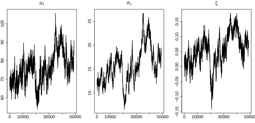
of simulated iid data. A total of 300 exceedances above a threshold u = 30 are simulated from a

Poisson process model withθ1 = (80,15,0.05). Figure 1 shows individual parameter chains for θk

from a random walk Metropolis scheme run for 50000 iterations with a burn-in of 1000 removed,

where k= 1 and a chosen m = 1. This figure shows the clear poor mixing of each component of

0 10000 30000 50000

60

70

80

90

100

µ1

0 10000 30000 50000

10

15

20

25

σ1

0 10000 30000 50000

−0.15

−0.10

−0.05

0.00

0.05

0.10

0.15

ξ

Figure 1: Random-walk Metropolis chains run for each component ofθ1.

We explore how reparameterising the model in terms ofmcan improve sampling performance. For

a general prior on the parameterisation of interest θk, denoted byπ(θk), Appendix B derives that

the prior on the transformed parameter space θm is

π(θm) =

m

k

−ξ

π(θk). (6)

In this example, independent Uniform priors are placed on µ1, logσ1 andξ, which gives

π(θ1)∝

1

σ1

; µ1 ∈_R, σ1 >0, ξ ∈_R. (7)

This choice of prior results in a proper posterior distribution, provided there are at least 4

thresh-old excesses (Northrop and Attalides, 2016). By finding a value of m that near-orthogonalises the

parameters of the posterior distribution π(θm|x), we can run an efficient MCMC scheme on θm

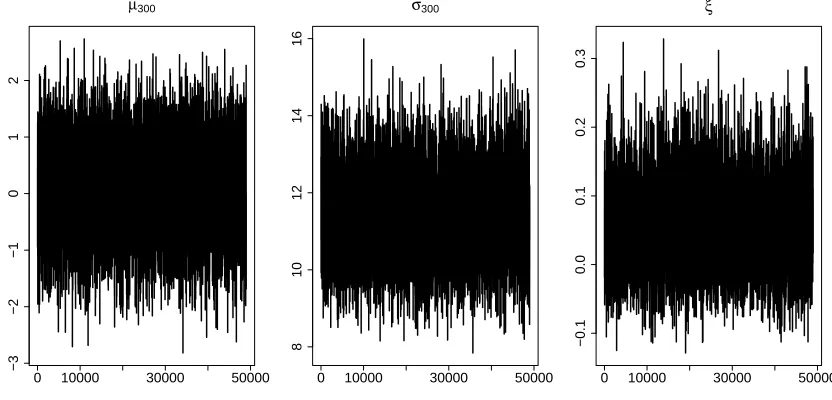
before transforming the samples to θk. It is noted in Wadsworth et al. (2010) that setting m to

be the number of exceedances above the threshold, i.e. m =r, improves the mixing properties of

the chain, as is illustrated in Figure 2. This is approximately equivalent to inference using a GP

model, as discussed in Section 1.

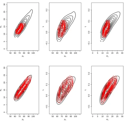
Given this choice of m, the MCMC scheme is run for θm before transforming to estimate the

posterior of θ1 using the mapping in (5), where k = 1 in this case. Figure 3 shows contour plots

of estimated joint posterior densities of θ1. It compares the samples from directly estimating the

0 10000 30000 50000

−3

−2

−1

0

1

2

µ300

0 10000 30000 50000

8

10

12

14

16

σ300

0 10000 30000 50000

−0.1

0.0

0.1

0.2

0.3

ξ

Figure 2: Random-walk Metropolis chains run for parameters θr, where r = 300 is the number of

exceedances in the simulated data.

a posterior sample for θ1. Figure 3 indicates that θ1 are highly correlated, with the result that

we only sample from a small proportion of the parameter space when exploring using independent

random walks for each parameter. This explains the poor mixing if we were to run the MCMC

without a transformation. It is clear that, after back-transforming to θ1, the reparameterisation

enables a more thorough exploration of the parameter space. However, while this transformation is

a useful tool in enabling an efficient Bayesian inference procedure, further investigation is necessary

in the choice ofm to achieve near-orthogonality of the parameter space and thus maximising the

efficiency of the MCMC procedure.

3

Choosing

m

optimally

As illustrated in Section 2, the choice ofmin the Poisson process likelihood can improve the

perfor-mance of the MCMC required to estimate the posterior density of model parametersθk. We desire

a value of msuch that near-orthogonality of θm is achieved, before using the expressions in (5) to

transform to the parameterisation of interest, e.g. θ1 or θny. As a measure of dependence, we use

the asymptotic expected correlation matrix of the posterior distribution of θm|x. In particular,

we explore how the off-diagonal components of the matrix, that is, the correlation between

param-eters, changes with m. The covariance matrix associated with θm|x can be derived analytically

by inverting the Fisher information matrix of the Poisson process log-likelihood (see Appendix C).

µ1 σ1

50 60 70 80 90 100

0

5

10

15

20

25

30

µ1

ξ

50 60 70 80 90 100

−0.1

0.0

0.1

0.2

σ1

ξ

0 5 10 15 20 25 30

−0.1

0.0

0.1

0.2

µ1 σ1

50 60 70 80 90 100

0

5

10

15

20

25

30

µ1

ξ

50 60 70 80 90 100

−0.1

0.0

0.1

0.2

σ1

ξ

0 5 10 15 20 25 30

−0.1

0.0

0.1

0.2

Figure 3: Contour plots of the estimated joint posterior of θ1 for 4000 iterations (top) and 49000

iterations (bottom) created from the transformed samples drawn from the MCMC procedure for

θm (in black) and samples ofθ1 drawn directly (in red).

Other choices for the measure of the dependence of the posterior could have been used, such as the

inverse of the Hessian matrix (or the expected Hessian matrix) of the log-posterior, evaluated at

the posterior mode. For inference problems with strong information from the data relative to the

prior there will be limited differences in the approach and similar values for the optimal mwill be

found. In contrast, if the prior is strongly informative and the number of threshold exceedances is

observed, rather than expected, Hessian may better represent the actual posterior distribution of

θm and deliver a choice ofm that better achieves orthogonalisation, see Efron and Hinkley (1978)

and Tawn (1987) respectively.

We prefer our choice of measure of dependence as for iid problems it gives closed form results for

mwhich can be used without the computational work required for other approaches, and this gives

valuable insight into the choice ofm. Furthermore, informative priors rarely arise in extreme value

problems, and so information in the data typically dominates information in the prior, particularly

around the posterior mode. It should be pointed out however, that the prior is used in the MCMC

so there is no loss of prior information in our approach. Also standard MCMC diagnostics should

be used even after the selection of an optimal m, so if the asymptotic posterior correlations differ

much from the posterior correlations, making our choice ofmpoor, this will be obvious and a more

complete but computationally burdensome analysis can be conducted using the methods described

above.

In this section, we use the data introduced in Section 2. For all integers m ∈ [1,500], maximum

likelihood estimates ˆθm are computed and pairwise correlations calculated by substituting ˆθm into

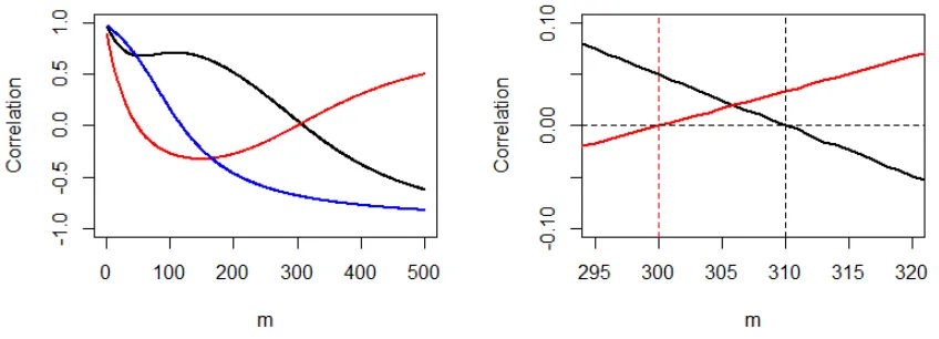
the expressions for the Fisher information matrix, in Appendix C, and taking the inverse. Figure 4

shows how parameter correlations change with the choice of m, illustrating that the asymptotic

posterior distributions of µm and ξ are orthogonal when m = r, the number of excesses above a

threshold, which explains the findings of Wadsworth et al. (2010).

Figure 4: Left: Estimated parameter correlations changing with m: ρµm,σm (black), ρµm,ξ (red),

ρσm,ξ (blue). Right: Expanded region of the graph showing ρµm,ξ = 0 for m close to r where

It is proposed that MCMC mixing can be further improved by minimising the overall correlation in

the asymptotic posterior distribution of θm. Therefore, we would like to find the value of m such

thatρ(θm) is minimised, whereρ(θm) is defined as

ρ(θm) =|ρµm,σm|+|ρµm,ξ|+|ρσm,ξ|, (8)

whereρµm,σmdenotes the asymptotic posterior correlation betweenµmandσmfor example. We also

Figure 5: Howρ(θm) changes withm (top left) and how correlations in each individual estimated

parameter, as measured byρµm, ρσm andρξ, change withm.

look at the sum of the asymptotic posterior correlation terms involving each individual parameter

estimate. For example, we define ρµm, the asymptotic posterior correlation associated with the

estimate ofµm, to be:

ρµm =|ρµm,σm|+|ρµm,ξ|. (9)

Figure 5 shows how the asymptotic posterior correlation associated with each parameter varies with

m. From Figure 5 we see that while ρµm is minimised at the value ofm for whichρµm,σm = 0 (see

minimum bym1 and the former bym2. In terms of the covariance function, this can be written as:

ACov(σm1, ξ|x) = ACov(µm2, σm2|x) = 0, (10)

where ACov denotes the asymptotic covariance. Figure 5 shows that m2 also minimises the total

asymptotic posterior correlation in the model.

One would expect that the values of m for which ρ(θm) is minimised would correspond to the

MCMC chain of θm with good mixing properties. We examine the effective sample size (ESS) as

a way of evaluating this objectively. ESS is a measure of the equivalent number of independent

iterations that the chain represents (Robert and Casella, 2009). MCMC samples are often

posi-tively autocorrelated, and thus are less precise in representing the posterior than if the chain was

independent. The ESS of a parameter chainφis defined as

ESSφ=

n

1 + 2P∞

i=1νi

, (11)

wheren is the length of the chain andνi denotes the autocorrelation in the sampled chain ofφat

lag i. In practice, the sum of the autocorrelations is truncated when νi drops beneath a certain

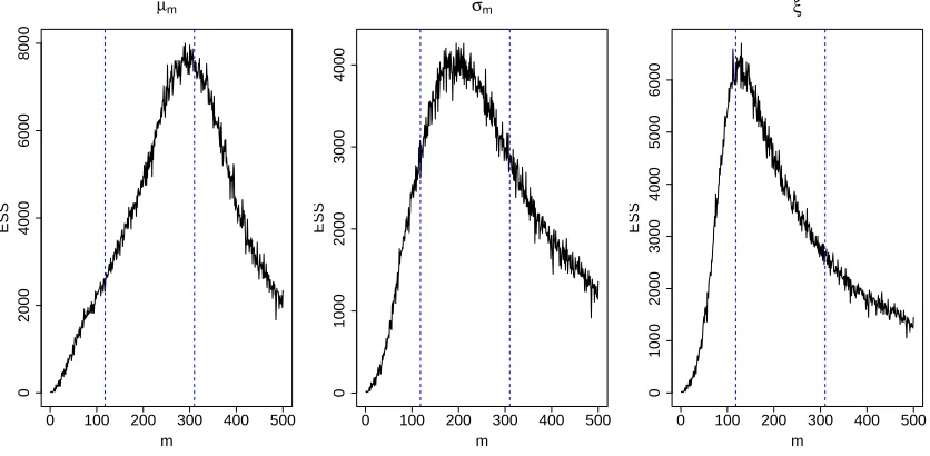
level. Figure 6 shows how ESS varies with m for each parameter in θm. For these data the ESS

follow a pattern we found to typically occur. We see that ESSµm is maximised atm=m2 due to

the near-orthogonality ofµm2 withσm2 andξ. We find that ESSσm is maximised form1 < m < m2,

as σm1 remains substantially postively correlated with µm1 and σm2 is negatively correlated with

ξ. Similarly, ESSξ is maximised at a value of m close to m1, but ξ is negatively correlated with

µm1, which explains the slight distortion. From these results, we postulate that a selection of

m in the interval (m1, m2) would ensure the most rapid convergence of the MCMC chain of θm,

thus enabling an effective sampling procedure from the joint posterior. Figure 6 shows clearly the

benefits of the proposed approach. For example, ESSµ310 = 7459.17 and ESSµ1 = 24.44, illustrating

that the former parameterisation is over 310 times more efficient than the latter. In addition, by

introducing the interval (m1, m2), this approach gives a degree of flexibility to the choice ofm and

giving a balance of mixing quality across the model parameters.

The quantitiesm1 andm2 can be found by numerical solution of the equations ACov(σm, ξ|x) = 0

and ACov(µm, σm|x) = 0 respectively, using the asymptotic covariance matrix of the posterior

of θm, which is given by the inverse of the Fisher information (see Appendix C). Approximate

0 100 200 300 400 500

0

2000

4000

6000

8000

µm

m

ESS

0 100 200 300 400 500

0

1000

2000

3000

4000

σm

m

ESS

0 100 200 300 400 500

0

1000

2000

3000

4000

5000

6000

ξ

m

ESS

Figure 6: How ESS varies with m for each parameter in θm. The blue dashed lines represent

m =m1 (left) and m= m2 (right) in the simulated data example, where m1 and m2 are defined

by property (10). In the calculations, the sum of the autocorrelations were truncated when the

autocorrelations in the chain drop below 0.05.

1985) applied to equations (10). This method yields the following approximations ofm1 and m2:

ˆ

m1 = r

(2ξ+ 1)1 + 2ξ+ (ξ+ 1) logh2₂ξ_ξ+3₊₁i

(2ξ+ 1)

3 + 2ξ−(ξ+ 1) log h

2ξ+3 2ξ+1

i (12)

ˆ

m2 = r2ξ

2_{+ 13ξ+ 8}

2ξ2_{+ 9ξ+ 8}. (13)

In practice, the values of ˆm1 and ˆm2 are estimated by using an estimate ofξ, such as the maximum

likelihood estimate. Figure 7 shows how ˆm1 and ˆm2 change relative to r for a range of ξ. This

illustrates that for negative estimates of the shape parameter, r is not a suitable candidate to be

the ‘optimal’ value of m as it is not in the range (m1, m2). In the simulated data used in this

section, although a selection of m =r is reasonable, Figure 6 shows that this may not be wise if

one was primarily concerned about sampling well fromξ, for example. In this case, ˆm2 is relatively

close tor, but Figure 7 shows that this is not the case for models with a larger positive estimate ofξ.

A simulation study was carried out to assess the suitability of expressions ˆm1 and ˆm2 as

approxi-mations tom1andm2 respectively. A total of 1000 Poisson processes were simulated with different

Figure 7: How ˆm1 and ˆm2 change as a multiple ofr with respect to ˆξ: ˆm1/r (black), ˆm2/r (red).

i = 1,2 always, while |mˆi−mi| < 0.01 for 78% and 88.2% of the time for i = 1,2 respectively.

Both quantities were compared to the performance of other approximations derived using Newton’s

method, which unlike Halley’s method does not account for the curvature in a function. Simulations

show that the root mean square errors are significantly smaller for estimates of mi using Halley’s

method (0.2% and 5% smaller than Newton’s method for i= 1,2 respectively). A summary of the

reparameterisation method is given in Algorithm 1.

Algorithm 1:Sampling from the posterior distribution of the Poisson process model

param-eters after reparameterising

Data: Threshold excesses x

Result: Samples from the posterior distributionπ(θk|x) 1 Choose parameterisation of interestθk;

2 if iid then

3 Obtain estimate of shape parameterξ using maximum likelihood, for example;

4 Compute ˆm₁ and ˆm₂ as defined in (12) and (13);

5 Choosem in range ( ˆm1,m2ˆ );

6 else

7 Choosem to be the value of mthat numerically solves ρ

µ(0)m,σm = 0;

4

Choosing

m

in the presence of non-stationarity

In many practical applications, processes exhibit trends or seasonal effects caused by underlying

mechanisms. The standard methods for modelling extremes of non-identically distributed

ran-dom variables were introduced by Davison and Smith (1990) and Smith (1989), using a

Pois-son process and Generalised Pareto distribution respectively. Both approaches involve setting

a constant threshold and modelling the parameters as functions of covariates. In this way, we

model the non-stationarity through the conditional distribution of the process on the covariates.

We follow the Poisson process model of Smith (1989) as the parameters are invariant to the

choice of threshold if the model is appropriate. We define the covariate-dependent parameters

θm(z) = (µm(z), σm(z), ξ(z)), for covariatesz. Often in practice, the shape parameterξis assumed

to be constant. A log-link is typically used to ensure positivity ofσm(z).

The process of choosing m is complicated when modelling in the presence of covariates. This is

partially caused by a modification of the integrated intensity measure, which becomes

Λ(A) =m

Z

z

1 +ξ(z)

u−µm(z)

σm(z)

−1/ξ(z)

g(z)dz, (14)

where g denotes the probability density function of the covariates, which is unknown and with

covariate spacez. The density termg is required as the covariates associated with exceedances of

the thresholdu are random. In addition, the extra parameters introduced by modelling covariates

increases the overall correlation in the model parameters.

For simplicity, we restrict our attention to the case of modelling when the location parameter is a

linear function of a covariate, that is,

µm(z) =µ(0)m +µ(1)m z, σm(z) =σm, ξ(z) =ξ,

where we centre the covariate z, as this leads to parameters µ(0)m and µ(1)m being orthogonal. Note

that the regression parameterµ(1)m is invariant to the choice ofm. A total of 233 excesses above a

threshold ofu= 15 are simulated from a Poisson process model with µ(0)₁ = 75,µ(1)₁ = 30,σ1 = 15,

ξ = −0.05. We choose g to follow an Exp(2) distribution, noting that one could also choose g to

be the density of a covariate that is used in practice. We impose an improper Uniform prior on the

regression parameterµ(1)₁ and set up the MCMC scheme in the same manner as in Section 3.

The objective remains to identify the value ofmthat achieves near-orthogonality of the parameters

samples back to the parameterisation of interest θk(z), which can be obtained as in (5) using the

relations

µ(0)_k = µ(0)_m −σm

ξ 1−

k m

−ξ!

µ(1)_k = µ(1)_m (15)

σk = σm

k m

−ξ

.

Figure 8: Contour plots of estimated posterior densities ofθ1(z) having sampled from the joint

pos-terior directly (red) and having transformed using (15) after reparameterising fromθ85(z) (black).

The complication of the integral term in the likelihood for non-identically distributed variables

means that it is no longer feasible to gain an analytical approximation for the optimal value ofm.

A referee has suggested a possible route to obtaining such expressions for m in the non-stationary

case, is by building on results in Attalides (2015) and using a non-constant threshold as in Northrop

and Jonathan (2011), but as this moves away from our constant threshold case we do not pursue

this. We therefore choose a value of m that minimises the asymptotic posterior correlation in the

model. Analogous to Section 3, the optimalmcoincides with the value ofm such thatρ_µ(0)

m,σm = 0.

Using numerical methods, we identify that this corresponds to a value ofm= 85 for the simulated

data example. Figure 8 shows contour plots of estimated posterior densities of θ1(z), comparing

the sampling from directly estimating the posteriorθ1(z) with that from transforming the samples

from the estimated posterior of θm(z) to give a sample from the posterior of θ1(z). From this

0 100 200 300 400 500

200

600

1000

1400

µ_m(0)

m

ESS

0 100 200 300 400 500

400

500

600

700

µ_m(1)

m

ESS

0 100 200 300 400 500

200

400

600

800

σm

m

ESS

0 100 200 300 400 500

0

500

1500

2500

ξ

m

ESS

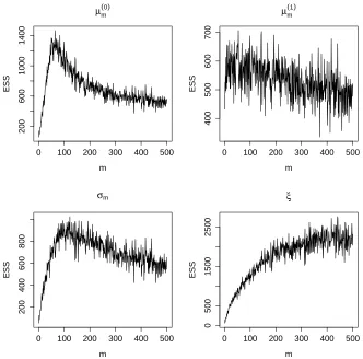
Figure 9: Effective sample size of each parameter chain of the MCMC procedure.

We again inspect the effective sample size for each parameter as a way of comparing the efficiency

of the MCMC under different parameterisations. Figure 9 shows how the effective sample size

varies with m for each parameter. This figure shows how the quality of mixing is approximately

maximised in µ(0)m for the value ofm that minimises the asymptotic posterior correlation. Mixing

for µ(1)m is consistent across all values of m. Interestingly, mixing in ξ increases as the value of m

increases. Without a formal measure for the quality of mixing across the parameters, it is found

that, when averaging the effective sample size over the number of parameters, the ESS is stable

with respect to m in the interval spanning from the value of m such that ρ_µ(0)

m,σm(0) = 0 and the

value of m such that ρ

σ(0)m,ξ = 0, like in Section 3. For a summary of how the reparameterisation

5

Case study: Cumbria rainfall

In this section, we present a study as an example of how this reparameterisation method can be

used in practice. In particular, we analyse data taken from the Met Office UKCP09 project, which

contains daily baseline averages of surface rainfall observations, measured in millimetres, in 25km

× 25km grid cells across the United Kingdom in the period 1958-2012. In this analysis, we focus

on a grid cell in Cumbria, which has been affected by numerous flood events in recent years, most

notably in 2007, 2009 and 2015. In particular, the December 2015 event resulted in an estimated

£5 billion worth of damage, with rain gauges reaching unprecedented levels. Many explanations

have been postulated for the seemingly increased rate of flooding in the North West of England,

including climate change, natural climate variability or a combination of both. The baseline

av-erage data for the flood events in December 2015 are not yet available, but this event is widely

regarded as being more extreme than the event in November 2009, the levels of which were reported

at the time to correspond to return periods of greater than 100 years. We focus our analysis on

the 2009 event, looking in particular at how a phase of climate variability, in the form of the North

Atlantic Oscillation (NAO) index, can have a significant impact on the probability of an extreme

event occurring in any given year.

Rainfall datasets on a daily scale are commonly known to exhibit a degree of serial correlation.

Analysis of autocorrelation and partial autocorrelation plots indicates that rainfall on day t is

dependent on the rainfall of the previous five days. In addition, the data may exhibit seasonal

effects. However, while serial dependence affects the effective sample size of a dataset, it does not

affect correlations between parameters, and is thus unlikely to influence the choice of m. For the

purposes of illustrating our method, we make the assumption for now that the rainfall observations

are iid and proceed with the method outlined in Section 3. We wish to obtain information about

the parameters corresponding to the distribution of annual maxima, i.e. θ55. Standard threshold

diagnostics (Coles, 2001) indicate a threshold of u = 15 is appropriate, which corresponds to the

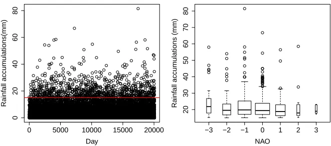
95.6% quantile of the data. There arer= 880 excesses aboveu (see Figure 10). We obtain bounds

m1 and m2, then choose a value m1 < m < m2 that will achieve near-orthogonality of the Poisson

process model parameters to improve MCMC sampling from the joint posterior distribution. We

obtain ˆξ = 0.087 using maximum likelihood when m=r, which we use to obtain approximations

for m1 and m2 as in (12) and (13). From this, we obtain ˆm1 ≈351 and ˆm2 ≈ 915. We checked

that ˆm1 and ˆm2 represent good approximations by solving equations (10) to obtain m1 = 350.82

and m2 = 914.96. Since r = 880 is contained in the interval (m1, m2), we choose m =r. We run

0 5000 10000 15000 20000

0

20

40

60

80

Day

Rainf

all accum

ulations(mm)

−3 −2 −1 0 1 2 3

20

30

40

50

60

70

80

NAO

Rainf

all accum

ulations (mm)

Figure 10: (Left) Daily rainfall observations in the Cumbria grid cell in the period 1958-2012. The

red line represents the extreme value threshold of u = 15. (Right) Boxplots of rainfall against

monthly NAO index.

transform the remaining samples using the mapping in (5), wherek= 55, to obtain samples from

the joint posterior ofθ55. The estimated posterior density for each parameter is shown in Figure 11.

To estimate probabilities of events beyond the range of the data, we can use the estimated

pa-rameters to estimate extreme quantiles of the annual maximum distribution. The quantity yN,

satisfying:

1/N = 1−G(yN), (16)

is termed theN-year return level, whereGis defined as in expression (2). The levelyN is expected

to be exceeded on average once every N years. By inverting (16) we get:

yN =

  

µ55−σ55_ξ [1− {−log(1−1/N)}−ξ] forξ6= 0

µ55−σ55log{−log(1−1/N)} forξ = 0.

(17)

The posterior density of the 100-year return level in Figure 11 is estimated by inputting the MCMC

samples of the model parameters into expression (17).

We use the same methodology to explore the effect of the monthly NAO index on the probability of

extreme rainfall levels in Cumbria. The NAO index describes the surface sea-level pressure

differ-ence between the Azores High and the Icelandic Low. The low frequency variability of the monthly

scale is chosen to represent the large scale atmospheric processes affecting the distribution of wind

and rain. In the UK, a positive NAO index is associated with cool summers and wet winters, while

Figure 11: Estimated posterior densities ofµ55,σ55,ξ and the 100-year return level.

further south to the Mediterranean region (Hurrell et al., 2003). In this analysis, we incorporated

the effect of NAO by introducing it as a covariate in the location parameter. The threshold of

u= 15 was retained for this analysis.

To obtain the value ofm that minimises the overall correlation in the model, we solve numerically

the equation ρ_µ(0)

m,σm = 0. We obtain a kernel density estimate of the NAO covariate, which

repre-sents g as defined in expression (14). We use this to obtain maximum likelihood estimates ˆθr(x).

These quantities are substituted into the Fisher information matrix. The matrix is then inverted

numerically to estimatem= 920. This represents a slight deviation from ˆm2 estimated during the

iid analysis. We would expect this as the covariate effect is small, as shown in Figure 12. This

example illustrates the benefit of numerically solving formwhen modelling non-stationarity, as the

range (m1, m2) estimated analytically during the iid analysis no longer contain the optimal value

We run an MCMC chain for θ920(x) for 50000 iterations before discarding the first 1000 samples

as burn-in. We transform the remaining MCMC samples to the annual maximum scale using the

mapping in (15) wherek= 55. Figure 12 indicates that NAO has a significantly positive effect on

the location parameter.

31 32 33 34 35 36 37 38

0.00

0.01

0.02

0.03

0.04

0.05

µ55

(0)

Density

0.0 0.5 1.0 1.5

0.00

0.01

0.02

0.03

0.04

0.05

µ55

(1)

Density

6 7 8 9 10 11

0.00

0.01

0.02

0.03

0.04

0.05

σ55

Density

0.00 0.05 0.10 0.15 0.20 0.25

0.00

0.01

0.02

0.03

0.04

ξ

Density

Figure 12: Estimated posterior densities ofµ(0)₅₅,µ(1)₅₅,σ55 and ξ.

We wish to estimate return levels relating to the November 2009 flood event, which is represented

by a value of 51.582mm in the dataset. Return levels corresponding to the distribution of November

maxima are shown in Figure 13. We can also use the predictive distribution in order to account for

both parameter uncertainty and randomness in future observations (Coles and Tawn, 1996). On

the basis of threshold excesses x= (x1, . . . , xn), the predictive distribution of a future November

maximumM is:

Pr{M ≤y|x}= Z

θ55

where

Pr{M ≤y|θ55}=

              

exp (

−₁₂1

1 +ξ

y−(µ(0)₅₅+µ(1)₅₅z) σ55

−1/ξ

+

)

where z is known

exp   

−₁₂1 Z

z

"

1 +ξ y−(µ (0) 55 +µ

(1) 55z) σ55

!#−1/ξ

+

gN(z)dz

  

where z is unknown,

(19)

where gN is the density of NAO in November and the integral is evaluated numerically using

adaptive quadrature methods. The integral in (18) can be approximated using a Monte Carlo

summation over the samples from the joint posterior ofθ55. From this, we estimate the predictive

probability of an event exceeding 51.582 in a typical November is 0.0112, with a 95% credible interval

of (0.0063,0.0185), which corresponds to an 89-year event, (54,158). For November 2009, when an

NAO index of −0.02 was measured, the probability of such an event was 0.0111, (0.0062,0.0184),

corresponding to a 90-year event, (54,161). For the maximum observed value of NAO in November,

with NAO = 3.04, the predictive probability of such an event is 0.0132, (0.0073,0.0214), which

corresponds to a 75-year flood event, (47,136). This illustrates the impact that different phases of

climate variability can have on the probabilities of extreme events.

Figure 13: Return levels corresponding to November maxima. The full line represents the posterior

Appendix

A

Proof:

µ

ˆ

=

u

when

m

=

r

We can write the full likelihood for parametersθr given a series of excesses{xi}above a threshold

u as:

L(θr) =L1×L2,

where L1 is the Poisson probability of r exceedances of u and L2 is the joint density of these r

exceedances, so that:

L1 =

1

r!

(

r

1 +ξ

u−µr

σr

−1/ξ

+ )r exp ( −r 1 +ξ

u−µr

σr

−1/ξ

+ ) , L2 = r Y i−1 1 σr 1 +ξ

xi−µr

σr

−1/ξ−1

+

1 +ξ

u−µr

σr

1/ξ

+ .

By defining Λ =h1 +ξu−µr_σr i

−1/ξ

+ and using identity (A), we can reparameterise the likelihood

in terms ofθ∗ = (Λ, ψu, ξ) to give:

L(θ∗)∝Λrexp{−rΛ}

r Y i=1 1 ψu 1 +ξ

xi−u

ψu

−1/ξ−1

+

Taking the log-likelihood and maximising with respect to Λ, we get:

l(θ∗) := logL(θ∗) =rlog ˆΛ−rΛˆ−rlogψu−

1

ξ −1

r X

i=1

log

1 +ξ

xi−u

ψu

+

∂l

∂Λ =

r

ˆ

Λ −r= 0,

which gives ˆΛ = 1. Then, by the invariance property of maximum likelihood estimators, ˆµr =u.

Using the identity

ψu=σm+ξ(u−µm),

which is invariant to choice of m, we get ˆσr = ˆψu. Because the ξ-dependent term in the

log-likelihood is identical to that in a GP log-log-likelihood, the maximum log-likelihood estimators of the two

models coincide.

B

Derivation of prior for inference on

θ

We define a joint prior on the parameterisation of interestθk. However, as we are making inference

density ofθm by using the density method for one-to-one bivariate transformations. Inverting (5)

to get expressions for µm and σm, i.e.

µm = µk−

σk

ξ

1−m

k

−ξ

=g1(µk, σk)

σm = σk

m

k

−ξ

=g2(µk, σk),

we can use this transformation to calculate the prior forθm.

π(θm) =π(µm, σm, ξ)

=π(µk, σk, ξ)|detJ|_µk=g−1

1 (µm,σm),σk=g

−1

2 (µm,σm),ξ=ξ,

where

detJ = ∂µm ∂µk ∂µm ∂σk ∂µm ∂ξ ∂σm ∂µk ∂σm ∂σk ∂σm ∂ξ ∂ξ ∂µk ∂ξ ∂σk ∂ξ ∂ξ = ∂µm ∂µk ∂µm ∂σk ∂µm ∂ξ

0 ∂σm_∂σk ∂σm_∂ξ

0 0 ∂ξ_∂ξ

= ∂σm

∂σk ∂ξ ∂ξ = m k −ξ .

Therefore, π(θm) = m_k

−ξ

π(θk).

C

Fisher information matrix calculations for iid random variables

The log-likelihood of the Poisson process model with parameterisation θm = (µm, σm, ξ) can be

expressed as

l(θm) =−m

1 +ξ

u−µm

σm

−1/ξ

+

−rlogσm−

1

ξ + 1

r X

j=1

log

1 +ξ

xj−µm

σm

+ ,

wherer is the number of exceedances ofX above the thresholdu. For simplicity, we drop the [·]₊

subscript in subsequent calculations. In order to produce analytic expressions for the asymptotic

covariance matrix, we must evaluate the observed information matrix ˆI(θm). For simplicity, we

definevm = u−µm_σm and zj,m= xj−µm

∂2l

∂µ2

m

= −m(ξ+ 1)

σ2

m

[1 +ξvm]−1/ξ−2+

ξ(ξ+ 1)

σ2

m r

X

j=1

[1 +ξzj,m]−2,

∂2l

∂σ2

m

= 2m

σ2

m

[1 +ξvm]−1/ξ−1vm−

m(ξ+ 1)

σ2

m

[1 +ξvm]−1/ξ−2v2m+ r

σ2

m

−2(ξ+ 1)

σ2

m r

X

j=1

[1 +ξzj,m]−1zj,m

+ξ(ξ+ 1)

σ2

m r

X

j=1

z_j,m2 [1 +ξzj,m]−2,

∂2l

∂ξ2 = −m[1 +ξvm]

−1/ξ

1

ξv

2

m[1 +ξvm]−2−

2

ξ3 log [1 +ξvm]

+ 2

ξ2[1 +ξvm]

−1_v

m+

1

ξ2 log [1 +ξvm]−

1

ξ[1 +ξvm]

−1_v

m 2# −2 ξ3 r X j=1

log [1 +ξzj,m] +

2

ξ2

r

X

j=1

[1 +ξzj,m]−1zj,m+

ξ+ 1

ξ r

X

j=1

[1 +ξzj,m]−2zj,m2 ,

∂2l

∂µm∂σm

= m

σ2

m

[1 +ξvm]−1/ξ−1−

m(ξ+ 1)

σ2

m

[1 +ξvm]−1/ξ−2vm

−ξ+ 1

σ2

m r

X

j=1

[1 +ξzj,m]−1+

ξ(ξ+ 1)

σ2

m r

X

j=1

[1 +ξzj,m]−2zj,m,

∂2l

∂µm∂ξ

= −m

σm

1

ξ2[1 +ξvm]

−1/ξ−1_{log [1 +ξv} m]−

ξ+ 1

ξ [1 +ξvm]

−1/ξ−2_v

m + 1 σm r X j=1

[1 +ξzj,m]−1

−ξ+ 1

σm

r

X

j=1

[1 +ξzj,m]−2zj,m,

∂2l

∂σm∂ξ

= −m

σm

vm

1

ξ2[1 +ξvm]

−1/ξ−1

log [1 +ξvm]−

ξ+ 1

ξ [1 +ξvm]

−1/ξ−2

vm + 1 σm r X j=1

[1 +ξzj,m]−1zj,m

−ξ+ 1

σm

r

X

j=1

[1 +ξzj,m]−2zj,m2

To obtain the Fisher information matrix, we take the expected value of each term in the observed

information with respect to the probability density of points of a Poisson process. LetZ = X_σm−µm,

and R be a random variable denoting the number of excesses ofX aboveu. The density of points

in the set Au can de defined by

f(x) = λ(x)

Λ(Au)

= [1 +ξz]

−1/ξ−1

whereλis a function denoting the rate of exceedance. Then, for example, EZ,R    R X j=1

[1 +ξzj,m]−2

  

= EREZ|R

   R X j=1

[1 +ξzj,m]−2

   = ER

n

REZ

n

[1 +ξZ]−2 oo

= ER

R[1 +ξvm]1/ξ

Z ∞

vm

[1 +ξz]−1/ξ−3dz

= m

2ξ+ 1[1 +ξvm]

−1/ξ−2

Following this process, we can write the Fisher information matrix I(θm) as:

E − ∂ 2_l ∂µ2 m

= m(ξ+ 1)

σ2

m

[1 +ξvm]−1/ξ−2−

mξ(ξ+ 1)

(2ξ+ 1)σ2 m

[1 +ξvm]−1/ξ−2,

E − ∂ 2_l ∂σ2 m

= −2m

σ2

m

[1 +ξvm]−1/ξ−1vm+

m(ξ+ 1)

σ2

m

[1 +ξvm]−1/ξ−2vm2 − r σ2 m + 2m σ2 m

[1 +ξvm]−1/ξ−1[1 + (ξ+ 1)vm]−

mξ

(2ξ+ 1)σ2 m

[1 +ξvm]−1/ξ−2

(2ξ2+ 3ξ+ 1)v2_m+ (4ξ+ 2)vm+ 2

, E −∂ 2_l ∂ξ2

= m[1 +ξvm]−1/ξ

1

ξv

2

m[1 +ξvm]−2−

2

ξ3 log [1 +ξvm]+

2

ξ2[1 +ξvm]

−1

vm+

1

ξ2log [1 +ξvm]−

1

ξ[1 +ξvm]

−1

2# +

2

ξ3[1 +ξvm]

−1/ξ

[ξ+ log [1 +ξvm]]−

2m

(ξ+ 1)ξ2[1 +ξvm]

−1/ξ−1

[1 + (ξ+ 1)vm]−

m

ξ(2ξ+ 1)[1 +ξvm]

−1/ξ−2

(2ξ2+ 3ξ+ 1)v_m2 + (4ξ+ 2)vm+ 2

, E − ∂ 2_l

∂µm∂σm

= m(ξ+ 1)

σ2

m

[1 +ξvm]−1/ξ−2vm−

mξ

(2ξ+ 1)σ2 m

[1 +ξvm]−1/ξ−2[1 + (2ξ+ 1)vm],

E

− ∂

2_l

∂µm∂ξ

= m

σm

1

ξ2[1 +ξvm]

−1/ξ−1_{log [1 +ξv} m]−

ξ+ 1

ξ [1 +ξvm]

−1/ξ−2_v

m

−

m

σm(ξ+ 1)

[1 +ξvm]−1/ξ−1+

m

σm(2ξ+ 1)

[1 +ξvm]−1/ξ−2[1 + (2ξ+ 1)vm],

E

− ∂

2_l

∂σm∂ξ

= m σm vm 1

ξ2[1 +ξvm]

−1/ξ−1

log [1 +ξvm] +

ξ+ 1

ξ [1 +ξvm]

−1/ξ−2

vm

−

m

σm(ξ+ 1)

[1 +ξvm]−1/ξ−1[1 + (ξ+ 1)vm] +

m

σm(2ξ+ 1)

[1 +ξvm]−1/ξ−2

(2ξ2+ 3ξ+ 1)v2_m+ (4ξ+ 2)vm+ 2

.

By inverting the Fisher information matrix using a technical computing tool like Wolfram

using the mapping in (5), we can get expressions for asymptotic posterior covariances.

ACov(µm, ξ) =

1

ξ2_r(ξ+ 1)σm

r

m

−ξ

ξ(ξ+ 1)r

m

ξ logr

m

−(2ξ+ 1)

r

m

ξ −1

ACov(µm, σm) =

1

ξ2_rσ

2 m

r

m

−ξr

m

ξ

(ξ+ 1) logr

m (ξ+ 1)ξlog

r

m

−3ξ−1+

ξ(ξ(ξ+ 2) + 3) + 1+ (ξ+ 1)(2ξ+ 1)logr

m

−1

ACov(σm, ξ) =

1

r(ξ+ 1)σm

(ξ+ 1) log r

m

−1

When m = r, ACov(µm, ξ) = 0. In addition, the m for which ACov(µm, σm) = 0 coincides with

the value ofmthat minimisesρθm as defined in (8). This root can easily be found numerically, but

an analytical approximation can be calculated using a one-step Halley’s method. By usingm =r

as the initial seed, and using the formula:

xn+1=xn−

f(xn)

f0_(x

n)−f(xn)f

00_(xn)

2f0_(xn)

we get the expression (13) for ˆm2 after one step. The quantity for ˆm1, given by expression (12)

requires two iterations of this method.

Acknowledgements

We gratefully acknowledge the support of the EPSRC funded EP/H023151/1 STOR-i Centre for

Doctoral Training, the Met Office and EDF Energy. We extend our thanks to Jenny Wadsworth

of Lancaster University and Simon Brown of the Met Office for helpful comments. We also thank

the Met Office for the rainfall data.

References

Attalides, N. (2015).Threshold-based extreme value modelling. PhD thesis, UCL (University College

London).

Chavez-Demoulin, V. and Davison, A. C. (2005). Generalized additive modelling of sample

ex-tremes. Journal of the Royal Statistical Society: Series C (Applied Statistics), 54(1):207–222.

Coles, S. G. (2001). An Introduction to Statistical Modeling of Extreme Values. Springer.

Coles, S. G. and Tawn, J. A. (1996). A Bayesian analysis of extreme rainfall data.Applied Statistics,

Cox, D. R. and Reid, N. (1987). Parameter orthogonality and approximate conditional inference

(with discussion). Journal of the Royal Statistical Society. Series B (Methodological), 49(1):1–39.

Davison, A. C. and Smith, R. L. (1990). Models for exceedances over high thresholds (with

discus-sion). Journal of the Royal Statistical Society. Series B (Methodological), 52(3):393–442.

Efron, B. and Hinkley, D. V. (1978). Assessing the accuracy of the maximum likelihood estimator:

Observed versus expected fisher information. Biometrika, 65(3):457–483.

Gander, W. (1985). On Halley’s iteration method.American Mathematical Monthly, 92(2):131–134.

Hills, S. E. and Smith, A. F. (1992). Parameterization issues in Bayesian inference. Bayesian

Statistics, 4:227–246.

Hurrell, J. W., Kushnir, Y., Ottersen, G., and Visbeck, M. (2003). An overview of the North

Atlantic oscillation. Geophysical Monograph-American Geophysical Union, 134:1–36.

Northrop, P. J. and Attalides, N. (2016). Posterior propriety in Bayesian extreme value analyses

using reference priors. Statistica Sinica, 26(2):721–743.

Northrop, P. J. and Jonathan, P. (2011). Threshold modelling of spatially dependent non-stationary

extremes with application to hurricane-induced wave heights. Environmetrics, 22(7):799–809.

Pickands, J. (1975). Statistical inference using extreme order statistics. The Annals of Statistics,

3(1):119–131.

Robert, C. and Casella, G. (2009). Introducing Monte Carlo Methods with R. Springer Science &

Business Media.

Roberts, G. O., Rosenthal, J. S., et al. (2001). Optimal scaling for various Metropolis-Hastings

algorithms. Statistical Science, 16(4):351–367.

Smith, R. L. (1985). Maximum likelihood estimation in a class of nonregular cases. Biometrika,

72(1):67–90.

Smith, R. L. (1987a). Discussion of “Parameter orthogonality and approximate conditional

infer-ence” by D.R. Cox and N. Reid. Journal of the Royal Statistical Society. Series B

(Methodolog-ical), 49(1):21–22.

Smith, R. L. (1987b). A theoretical comparison of the annual maximum and threshold approaches

Smith, R. L. (1989). Extreme value analysis of environmental time series: an application to trend

detection in ground-level ozone. Statistical Science, 4(4):367–377.

Stephenson, A. (2016). Bayesian inference for extreme value modelling. Extreme Value Modeling

and Risk Analysis: Methods and Applications, pages 257–280.

Tawn, J. A. (1987). Discussion of “Parameter orthogonality and approximate conditional inference”

by D.R. Cox and N. Reid. Journal of the Royal Statistical Society. Series B (Methodological),

49(1):33–34.

Wadsworth, J. L., Tawn, J. A., and Jonathan, P. (2010). Accounting for choice of measurement